The Analytic Hierarchy Process

Multicriteria Decision Making for Vehicle Routing

Breno A. Beirigo

Date

2026-08-14

A principled introduction to pairwise comparison, priority weights, and consistency.

Outline

1. Why AHP? — The problem of multicriteria decisions
2. Structuring the hierarchy — Goals, criteria, alternatives
3. The fundamental scale — Pairwise comparisons
4. From judgments to weights — Why simple methods break down
5. The eigenvector solution — A natural derivation
6. Consistency — Detecting contradictory judgments
7. Application to VRP — Worked example with two KPIs
8. Discussion — Strengths, limitations, and extensions

This presentation introduces the Analytic Hierarchy Process (AHP) as proposed by Saaty (1990) and adapts it to a transportation and vehicle routing context. The AHP is “a multicriteria decision making approach in which factors are arranged in a hierarchic structure” (Saaty, 1990, p. 9). We will see how it can help logistics planners choose among competing route plans when multiple, possibly conflicting, KPIs must be balanced.

Special emphasis is placed on building intuition for why the eigenvector is the right tool — not as a black box from linear algebra, but as the natural consequence of wanting to account for all direct and indirect comparisons simultaneously.

The Decision Problem

In operations research, we often face decisions where no single objective tells the whole story.

In VRP, a planner must balance, for example:

• Total travel distance (cost)
• Driver workload equity
• Number of vehicles used
• Customer time-window violations
• Employee satisfaction Turnover risk

The trap of arbitrary scoring:

Assigning ad-hoc weights and normalizing arbitrary numbers is “mere number crunching”: it can produce any desired answer (Saaty 1990).

Saaty (1990, p. 10) warns forcefully against ad-hoc scoring: “If a decision support theory is to be trustworthy there must be uniqueness in the representation of judgments, the scales derived from these judgments, and the scales synthesized from the derived scales.”

He further observes that “among the various number crunching practices, the most objectionable one is to assign any set of numbers to judgments on alternatives under a particular criterion, and then normalize these numbers” (p. 10). This is precisely what happens when logistics planners eyeball a set of route plans and assign scores from 1 to 10 on different KPIs without any formal structure. The AHP provides a principled alternative.

Why Not Just Normalize and Assign Weights?

Faced with multiple KPIs with different units and scales, a candidate approach is to normalize each KPI to \([0,1]\) and then assign weights to combine them into a single score:

\[ \text{Score} = w_1 \cdot \text{Distance}_{\text{norm}} + w_2 \cdot \text{Balance}_{\text{norm}} + w_3 \cdot \text{Satisfaction}_{\text{norm}} \]

However, some criteria are inherently ordinal (they express a rank order but no meaningful quantity). Examples include:

• Customer satisfaction ratings (e.g., “Good,” “Acceptable,” “Poor”)
• Employee performance levels (e.g., “Exceeds expectations,” “Meets expectations,” “Needs improvement”)
• Risk levels (e.g., “Low,” “Medium,” “High”)

“Among the various number crunching practices, the most objectionable one is to assign any set of numbers to judgments on alternatives under a particular criterion, and then normalize these numbers (by multiplying them by a constant that is the reciprocal of their sum). Generally, different sets of numbers are used to scale the judgments for the alternatives under different criteria. All the new normalized sets now lie in the interval [0, 1], no matter what scale they originally came from, and can be passed off to the uninitiated as comparable. The appealing part of this practice is that the numbers have an apparently uniform underlying structure and look not unlike probabilities. Thus they go unchallenged by the decision maker and are then manipulated by the consultant or facilitator who weights and adds them to find the most preferred alternative. Note that when the initial numbers assigned before normalization are ordinals, arbitrary numbers that preserve order but carry no information about differences or ratios of relative magnitudes, the resulting transformation produces a new set of ordinals lying between zero and one and you can be sure only that it preserves the same order. The operations of weighting and adding cannot then be meaningful because it is very likely that different results will be produced for different choices of the ordinal numbers. By a judicious choice of ordinals one can make an alternative that is dominant on even one criterion, no matter how unimportant that criterion may be, have the largest value after weighting and adding and thus turn out to be the most preferred. Any method such as this is not a decision theory but an approach that can mislead people”

Example: Encoding Ordinal Data

A logistics planner rates each route plan’s driver acceptance as Good, Acceptable, or Poor. Everyone agrees on the ranking:

\[\text{Good} \;>\; \text{Acceptable} \;>\; \text{Poor}\]

But to plug these into a weighted sum, we must assign numbers. And there is no principled way to do it.

This motivating example is inspired by Saaty’s warning (1990, p. 10): “By a judicious choice of ordinals one can make an alternative that is dominant on even one criterion, no matter how unimportant that criterion may be, have the largest value after weighting and adding and thus turn out to be the most preferred.”

Driver satisfaction is a realistic ordinal variable in VRP. A planner can rank routes as “good,” “acceptable,” and “poor” — but the question “how much better is good than acceptable?” has no objective answer. Is the gap between good and acceptable the same as between acceptable and poor? Twice as large? Half? There is simply no fact of the matter, because the labels carry rank information only.

The Ordinal Trap: Arbitrary Encodings

Consider two plausible encodings of the same ordinal data in Table 1, where:

• Distance: measured in kilometers (lower is better)
• Workload balance: measured as standard deviation of driver hours (lower is better)
• Employee satisfaction: measured qualitatively as Good > Acceptable > Poor.

Table 1: Same qualitative labels encoded two ways: evenly spaced (A) vs. top-heavy (B).

Plan	Distance (km)	Worload Balance (h)	Employee Satisfaction	Encoding A	Encoding B
P1	135	0.9	Good	3	3
P2	142	0.4	Acceptable	2	2.8
P3	158	1.8	Poor	1	1

Which encoding is better?

Both encodings respect Good > Acceptable > Poor. The only difference is where “Acceptable” sits between Good and Poor.

• Encoding A says: Acceptable is halfway between Good and Poor.
• Encoding B says: Acceptable is almost as good as Good.

Neither is wrong; the labels simply don’t carry distance information.

This is the crux of the problem. The planner said “Acceptable.” They did not say “exactly one unit below Good” or “almost as good as Good.” Both encodings are faithful to the original ordinal judgment — they preserve the order — but they impose different cardinal assumptions.

In practice, different analysts will choose different encodings. Encoding A (1, 2, 3) feels “natural” because the numbers are evenly spaced. But why should the gap between Good and Acceptable be the same as between Acceptable and Poor? A planner might well feel that Good and Acceptable are close while Poor is far below both — that’s Encoding B.

The fact that reasonable people can disagree on the encoding, while agreeing completely on the ranking, is exactly why ordinal data cannot be meaningfully weighted and summed.

The Ordinal Trap: Same Labels, Different Winner

Let’s see what happens when we:

1. Normalize each column to \([0,1]\) (min-max)
2. Assign weights to each criterion and compute a weighted sum for each plan.

We will consider weights: \(w_{\text{dist}} = 0.3\), \(w_{\text{bal}} = 0.4\), \(w_{\text{sat}} = 0.3\).

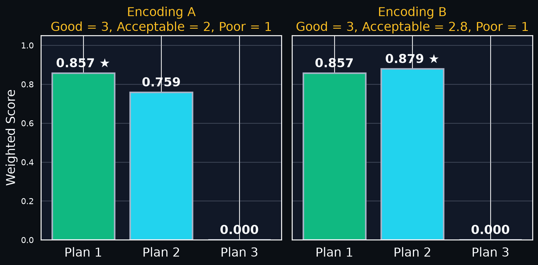
Figure 1 shows the results for both encodings.

Figure 1

Outcome: With Encoding A, Plan 1 wins. With Encoding B, Plan 2 wins.

Let’s trace through what happens:

Encoding A (Good=3, Acceptable=2, Poor=1 — evenly spaced): Plan 2’s satisfaction normalizes to \((2 - 1)/(3 - 1) = 0.50\). Despite Plan 2’s excellent workload balance (normalized to 1.0), the large satisfaction penalty (0.50 vs 1.00) keeps it behind Plan 1. Final scores: Plan 1 = 0.857, Plan 2 = 0.759.

Encoding B (Good=3, Acceptable=2.8, Poor=1 — top-heavy): Now Plan 2’s satisfaction normalizes to \((2.8 - 1)/(3 - 1) = 0.90\). The gap between Good and Acceptable shrinks from 0.50 to 0.10. Plan 2’s strong balance advantage (1.0 vs 0.643) is no longer overwhelmed by the satisfaction penalty. Final scores: Plan 1 = 0.857, Plan 2 = 0.879. The winner flips.

The mechanism is clear: the encoding determines how much “credit” Plan 2 gets for being Acceptable rather than Good. With even spacing, the penalty is 50% of the satisfaction range. With top-heavy spacing, it’s only 10%. Since both encodings are equally defensible readings of the ordinal label “Acceptable,” the decision is not determined by the planner’s actual preferences — it’s determined by an analyst’s arbitrary coding choice.

Saaty (1990, p. 10) identifies this precisely: “among the various number crunching practices, the most objectionable one is to assign any set of numbers to judgments on alternatives under a particular criterion, and then normalize these numbers.”

This is why MCDM methods like AHP and BWM exist: they derive ratio-scale weights from structured pairwise comparisons. Instead of encoding “Acceptable” as a number, AHP asks: “How many times more satisfying is Plan 1 than Plan 2 to the drivers?” This pairwise ratio judgment produces a meaningful scale that does not depend on arbitrary encoding choices.

Why Not Just Normalize and Assign Weights?

• Faced with multiple KPIs with different units and scales, a candidate approach is to normalize each KPI to \([0,1]\) and then assign weights to combine them into a single score.
• Normalizing has a critical flaw: ordinal scales (e.g., 1 to 10) only preserve order, not meaningful ratios. For example:
  • Consider a scale of 1 to 10 for employee satisfaction. The difference between 1 and 2 is not necessarily the same as the difference between 9 and 10. Normalizing these scores to \([0,1]\) would give equal weight to all differences, which may not reflect the true importance of changes in satisfaction.

Weighting and adding such numbers can produce any ranking depending on the choice of ordinals.

The ordinal trap

When initial numbers are ordinals (preserving only order), normalizing them to \([0,1]\) preserves only order — not meaningful ratios. Weighting and adding such numbers can produce any ranking depending on the choice of ordinals.

Example: Two route plans scored on “distance” as 3 and 7 (ordinal). Normalizing gives 0.30 and 0.70. But scoring them as 1 and 9 gives 0.10 and 0.90 — same order, wildly different weights.

\(\Rightarrow\) We need a method that produces ratio scales from judgments.

Saaty makes the point vividly: “By a judicious choice of ordinals one can make an alternative that is dominant on even one criterion, no matter how unimportant that criterion may be, have the largest value after weighting and adding and thus turn out to be the most preferred. Any method such as this is not a decision theory but an approach that can mislead people.” (Saaty, 1990, p. 10)

The AHP is “rigorously concerned with the scaling problem and what sort of numbers to use, and how to correctly combine the priorities resulting from them” (p. 10). It produces ratio scales — scales with a meaningful zero and where ratios between measurements are interpretable.

Structuring the Hierarchy

Three levels:

1. Goal: Select the best VRP solution
2. Criteria: The KPIs we care about
3. Alternatives: Candidate route plans

Saaty (1990, p. 9) describes the hierarchy construction: “In the Analytic Hierarchy Process we arrange these factors, once selected, in a hierarchic structure descending from an overall goal to criteria, subcriteria and alternatives in successive levels.”

He emphasizes that the hierarchy serves two purposes: “It provides an overall view of the complex relationships inherent in the situation; and helps the decision maker assess whether the issues in each level are of the same order of magnitude, so he can compare such homogeneous elements accurately.” (p. 9)

A key insight is that “a hierarchy does not need to be complete, that is, an element in a given level does not have to function as an attribute (or criterion) for all the elements in the level below.” (p. 9). In our VRP context, we keep it simple with two criteria and three alternatives, but in practice the hierarchy could include subcriteria (e.g., under “workload balance”: max hours per driver, variance of hours, number of overtime violations).

The Fundamental Scale

Saaty’s fundamental scale adapted for VRP criteria comparison

Intensity	Definition	VRP Interpretation
1	Equal importance	Both KPIs matter equally
3	Moderate importance	Distance is moderately more important than balance
5	Strong importance	Distance is strongly more important
7	Very strong importance	Distance demonstrably dominates
9	Extreme importance	Distance is the sole practical concern
2,4,6,8	Intermediate values	Compromise between adjacent judgments

Reciprocal property

If criterion \(i\) is rated \(a_{ij}\) relative to criterion \(j\), then \(a_{ji} = 1/a_{ij}\).

Saaty (1990, p. 15, Table 1) presents the fundamental scale with intensities 1 through 9. He notes that “this scale has been validated for effectiveness, not only in many applications by a number of people, but also through theoretical comparisons with a large number of other scales.”

The reciprocal property is fundamental: “If activity \(i\) has one of the above numbers assigned to it when compared with activity \(j\), then \(j\) has the reciprocal value when compared with \(i\).” (Saaty, 1990, p. 15)

Saaty also mentions that “when the elements being compared are closer together than indicated by the scale, one can use the scale 1.1, 1.2, …, 1.9” (p. 16). This is useful when comparing, say, two route plans that are very close in total distance.

The connection to George Miller’s “magical number seven, plus or minus two” is important: Saaty recommends comparing no more than about 7–9 elements at a time to maintain consistency. This is why clustering (Section 7 of the paper) becomes essential for large problems.

From Judgments to Weights: The Core Challenge

Suppose a planner compares three route plans on total distance and gives these pairwise ratios:

\[ A = \begin{pmatrix} 1 & 3 & 5 \\ 1/3 & 1 & 2 \\ 1/5 & 1/2 & 1 \end{pmatrix} \]

The question: What weight vector \(\mathbf{w} = (w_1, w_2, w_3)\) best represents these judgments?

This is not obvious. Several methods come to mind:

1. Normalize any column of \(A\)
2. Average the normalized columns (row geometric mean)
3. Something else?

Let’s see what happens when judgments are perfectly consistent — and when they’re not.

This is the central methodological question of AHP. We have a matrix of pairwise ratios and want to extract a weight vector. The answer seems straightforward, but as we’ll see, the choice of method matters when judgments contain contradictions.

Saaty (1990, p. 12) sets up the problem using a stone-weighing analogy: “Assume that we are given \(n\) stones, \(A_1, \ldots, A_n\), whose weights \(w_1, \ldots, w_n\), respectively, are known to us. Let us form the matrix of pairwise ratios whose rows give the ratios of the weights of each stone with respect to all others.”

The Easy Case: Perfect Consistency

If the planner is perfectly consistent, every ratio is exact: \(a_{ij} = w_i / w_j\).

Then \(a_{ik} = a_{ij} \cdot a_{jk}\) for all \(i, j, k\). (Transitivity of ratios)

Example: If Plan A is 3× better than B, and B is 2× better than C, then A must be 6× better than C.

\[ A_{\text{consistent}} = \begin{pmatrix} 1 & 3 & 6 \\ 1/3 & 1 & 2 \\ 1/6 & 1/2 & 1 \end{pmatrix} \]

Every method agrees for this matrix:

• Normalize column 1: \((0.667, 0.222, 0.111)\)
• Normalize column 2: \((0.667, 0.222, 0.111)\)
• Normalize column 3: \((0.667, 0.222, 0.111)\)

All columns give the same answer!

Note

When judgments are consistent, any column (normalized) recovers the true weights. The matrix has rank 1 — all columns carry the same information.

Saaty (1990, p. 12) states: “It is clear that if we are given the comparison matrix \(A\), we can recover the scale. In this case the solution is the normalized version of any column of \(A\).”

This is the key insight: a consistent matrix is fully determined by any single column (or row). Mathematically, it has rank 1. Every row is a scalar multiple of every other row. The consistency condition \(a_{jk} = a_{ik}/a_{ij}\) (Saaty, 1990, p. 12, Eq. 1) ensures this.

At this point students might wonder: if any column works, why do we need anything fancier? The answer is that real judgments are never perfectly consistent.

The Hard Case: Inconsistent Judgments

Now suppose the planner says:

• A is 3× better than B ✓
• B is 2× better than C ✓
• A is 5× better than C ⚠️ (should be 6 if consistent)

\[ A_{\text{inconsistent}} = \begin{pmatrix} 1 & 3 & 5 \\ 1/3 & 1 & 2 \\ 1/5 & 1/2 & 1 \end{pmatrix} \]

Now the columns disagree:

Method	\(w_1\)	\(w_2\)	\(w_3\)
Normalize column 1	0.652	0.217	0.130
Normalize column 2	0.667	0.222	0.111
Normalize column 3	0.625	0.250	0.125

Which column should we trust? None of them — each reflects only part of the information.

This is where the core pedagogical challenge lies. With inconsistency, each column of the matrix gives a slightly different weight vector. Simply picking one column would be arbitrary — it would ignore the information in the other columns.

One naive response is to average the columns. That’s reasonable but, as we’ll see, it doesn’t account for all the information in the matrix. The matrix contains not just direct comparisons (column by column) but also indirect comparisons — information about how alternatives relate through intermediate comparisons.

The inconsistency here is small (5 instead of 6), but it illustrates the fundamental problem. In practice, with many criteria and alternatives, inconsistencies accumulate and the choice of method matters more.

Why Not Just Average?

A natural first idea: average the normalized columns, or equivalently, compute row sums and normalize.

This works reasonably well in many cases. But it misses something important.

The problem with row-sum averaging

Row sums only capture one-step dominance: how much does Plan A directly dominate each other plan?

But dominance can also be indirect.

Analogy from sports: In a tournament, Team A might not play Team C directly. But if A beat B, and B beat C, we learn something about A vs. C.

The comparison matrix \(A\) is like a weighted tournament. We need a method that considers all paths of comparison, not just direct ones.

This is the critical conceptual step. Saaty (1990, p. 18–19) develops this idea through dominance walks:

“The matrix \(A\) captures only the dominance of one alternative over every other in one step. But an alternative can dominate a second by first dominating a third alternative and then the third dominates the second. Thus, the first alternative dominates the second in two steps.”

The analogy to tournaments and sports is very effective pedagogically. Students who follow rankings in football or tennis understand intuitively that “strength of schedule” matters — you get more credit for beating a team that itself has beaten strong teams. The eigenvector method captures exactly this: it weights each comparison by the importance of the alternatives being compared.

Saaty further explains: “It is known that the result for dominance in two steps is obtained by squaring the pairwise comparison matrix. Similarly, dominance can occur in three steps, four steps and so on, the value of each is obtained by raising the matrix to the corresponding power.” (Saaty, 1990, p. 18–19)

Dominance Walks: The Key Idea

Think of the comparison matrix as a directed graph with weighted edges:

Direct (1-step) dominance: Row sums of \(A\)

Indirect (2-step) dominance: Row sums of \(A^2\)

A dominates C through B: \(3 \times 2 = 6\)

All-step dominance: Row sums of \(A + A^2 + A^3 + \cdots\)

This captures the total influence of each alternative through every possible comparison path.

The big question

Does this infinite sum converge to something meaningful?

Yes — it converges to the principal eigenvector of \(A\).

Saaty (1990, p. 19) formulates this as a graph-theoretic concept:

“We can think of the alternatives as the nodes of a directed graph. With every directed arc from node \(i\) to node \(j\) (which need not be distinct), is associated a nonnegative number \(a_{ij}\) of the dominance matrix.”

He defines a \(k\)-walk and proves (Theorem 3) that the average dominance along all walks converges to the principal eigenvector.

The pedagogical power of this framing is enormous: students don’t need to know eigenvalue theory to understand that we want a ranking that accounts for all comparison paths, not just direct ones. The eigenvector emerges as the answer to a well-motivated question, rather than as an imposed algebraic technique.

The tournament analogy works well here. In the analogy: - \(A\) is like the matrix of match results - \(A^2\) tells you about two-game paths (A beat B, B beat C) - \(A^k\) tells you about \(k\)-game paths - The eigenvector is the “true strength” rating that accounts for all paths

The Eigenvector Emerges Naturally

Definition (Saaty, 1990): The total dominance of alternative \(i\) across walks of length \(1, 2, \ldots, m\) is:

\[ t_m = \frac{1}{m} \sum_{k=1}^{m} \frac{A^k \mathbf{e}}{\mathbf{e}^T A^k \mathbf{e}} \]

where \(\mathbf{e} = (1, 1, \ldots, 1)^T\) (so \(A^k \mathbf{e}\) gives the row sums of \(A^k\)).

Theorem 3 (Saaty, 1990): As \(m \to \infty\), this converges to \(\mathbf{w}\), the solution of:

\[A \mathbf{w} = \lambda_{\max} \mathbf{w}\]

In plain language

The eigenvector is the unique ranking that is self-consistent with all direct and indirect comparisons in the matrix. It’s not an arbitrary algebraic choice — it’s the answer to the question “what ranking respects all comparison paths?”

Saaty (1990, p. 19) proves this as Theorem 3: “The dominance of each alternative along all walks \(k\), is given by the solution of the eigenvalue problem \(Aw = \lambda_{\max} w\).”

The proof uses Cesàro summability: since \(s_k = A^k e / (e^T A^k e) \to w\) as \(k \to \infty\) (by the Perron–Frobenius theorem), the Cesàro mean \(t_m = (1/m) \sum s_k\) converges to the same limit.

This is the “aha” moment for students: the eigenvector is not a tool we borrow from linear algebra and apply blindly — it is the natural outcome of asking “what priority vector accounts for all paths of comparison?”

Saaty also notes: “The solution of the eigenvalue problem is obtained by raising the matrix \(A\) to a sufficiently large power then summing over the rows and normalizing to obtain the priority vector \(w = (w_1, \ldots, w_n)^T\). The process is stopped when the difference between components of the priority vector obtained at the \(k\)-th power and at the \((k+1)\)st power is less than some predetermined small value.” (Saaty, 1990, p. 19)

This computational procedure (the power method) is itself illuminating: you literally compute \(A, A^2, A^3, \ldots\) and watch the normalized row sums converge. Students can do this by hand for a \(3 \times 3\) matrix.

Seeing It Work: Power Method by Hand

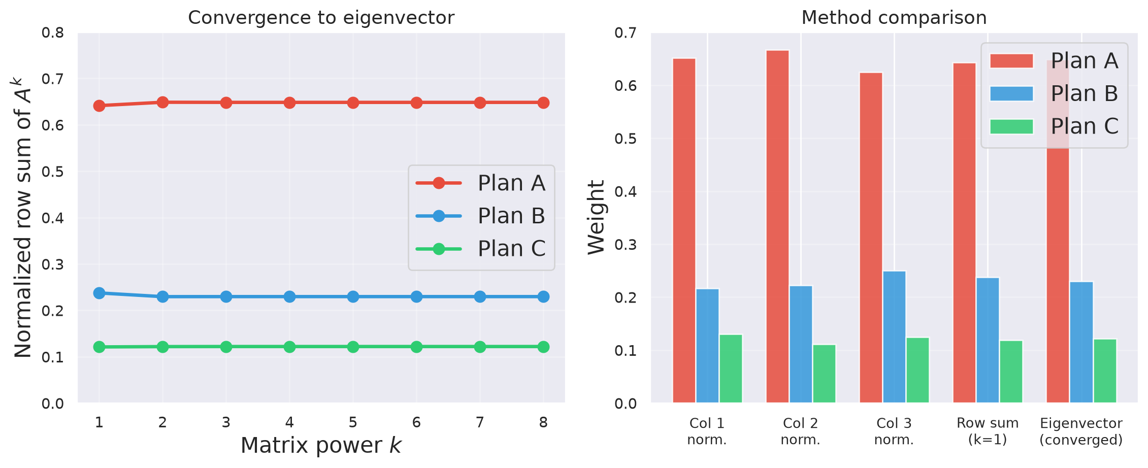
Eigenvector (converged): [0.6483 0.2297 0.122 ]

The left panel shows the key insight visually: as we raise \(A\) to higher and higher powers, the normalized row sums converge to fixed values. Those fixed values are the principal eigenvector.

At \(k=1\), we get simple row-sum averaging. At \(k=2\), we incorporate two-step dominance. By about \(k=4\) or \(k=5\), the values have essentially converged.

The right panel compares different methods side by side. Notice how the individual column normalizations disagree with each other (because of inconsistency), while the eigenvector provides a principled synthesis of all the information.

Importantly, for this nearly-consistent matrix, all methods give similar answers. The differences become more pronounced as inconsistency increases. Saaty (1990, p. 19) discusses five different methods and notes: “All methods yield the same answer when the matrix is consistent.”

Why the Eigenvector and Not Some Other Method?

Saaty (1990, p. 19) lists five ways to derive priorities from the comparison matrix:

1. Eigenvector — captures dominance through all walk lengths
2. Row sum average — captures only direct (1-step) dominance
3. Normalized column average — averages multiple partial views
4. Least squares — minimizes sum of squared deviations
5. Logarithmic least squares (geometric mean) — minimizes product-form deviations

All agree for consistent matrices. For inconsistent ones, the eigenvector is special:

Saaty’s argument (p. 19)

“So long as inconsistency is tolerated, dominance is the basic theoretical concept for deriving a scale and no other method qualifies.”

The eigenvector is the only method that accounts for the full structure of indirect comparisons. Row averages see one step; the eigenvector sees infinitely many.

Saaty (1990, p. 19) is quite emphatic about this: “We argue that so long as inconsistency is tolerated, dominance is the basic theoretical concept for deriving a scale and no other method qualifies. In addition, a counterexample has been provided in which the [logarithmic least squares] method not only does not generate a good approximation, but also reverses rank.”

He also concedes pragmatically: “It may be that the arithmetic of a method is simpler than that used to obtain the eigenvector, but that no longer matters, because of the widespread use of the computer.” (Saaty, 1990, p. 19–20)

For teaching purposes, the key message is: - Simple methods (row averages, column averages) work as approximations for nearly-consistent matrices - The eigenvector is the theoretically correct method because it captures the full dominance structure - In practice, the differences are often small, but when they matter (high inconsistency, close alternatives), the eigenvector is more reliable

An additional point from Saaty: “In reference [7] we pointed out that the logarithmic least squares solution coincides with the principal right eigenvector solution for matrices of order \(n = 3\), which is the first value of \(n\) for which inconsistency is possible.” (Saaty, 1990, p. 19). So for our 3×3 examples, the geometric mean method and the eigenvector actually agree.

Now: What Is Consistency, Exactly?

A planner comparing three route plans says:

Consistent judgments ✅

• A is 3× better than B
• B is 2× better than C
• A is 6× better than C

The indirect path (3 × 2 = 6) matches the direct judgment (6).

Inconsistent judgments ⚠️

• A is 3× better than B
• B is 2× better than C
• A is 5× better than C

The indirect path says 6, but the direct judgment says 5. Something doesn’t add up.

Consistency = transitivity of ratios

A matrix is consistent when \(a_{ij} \cdot a_{jk} = a_{ik}\) for all \(i, j, k\).

This means: every indirect comparison path gives the same answer as the direct comparison.

Saaty (1990, p. 12) formalizes this: “In addition, \(A\) is consistent because the following condition is satisfied: \(a_{jk} = a_{ik}/a_{ij}\), \(i, j, k = 1, \ldots, n\).” (Equation 1)

This is the ratio-scale version of transitivity. In ordinal terms, transitivity means: if A > B and B > C, then A > C. In ratio terms, it’s stronger: if A/B = 3 and B/C = 2, then A/C must equal 6.

Perfect consistency is unrealistic for human judgments. As Saaty notes, the relevant question is not whether we are consistent, but how close to consistent we are. Small deviations from transitivity are acceptable; large ones suggest the decision-maker has contradictory preferences that need revision.

The condition can also be stated as: “the entire matrix can be constructed from a set of \(n\) elements which form a chain (or more generally, a spanning tree, in graph-theoretic terminology) across the rows and columns.” (Saaty, 1990, p. 13). In other words, if you know \(n-1\) independent ratios, all other ratios are determined.

Why Does Inconsistency Matter?

Consider a logistics manager who says:

• Route A is much better than Route B on distance (7×)
• Route B is much better than Route C on distance (7×)
• Route C is better than Route A on distance (3×)

This is circular: A ≫ B ≫ C > A.

\[ A_{\text{bad}} = \begin{pmatrix} 1 & 7 & 1/3 \\ 1/7 & 1 & 7 \\ 3 & 1/7 & 1 \end{pmatrix} \]

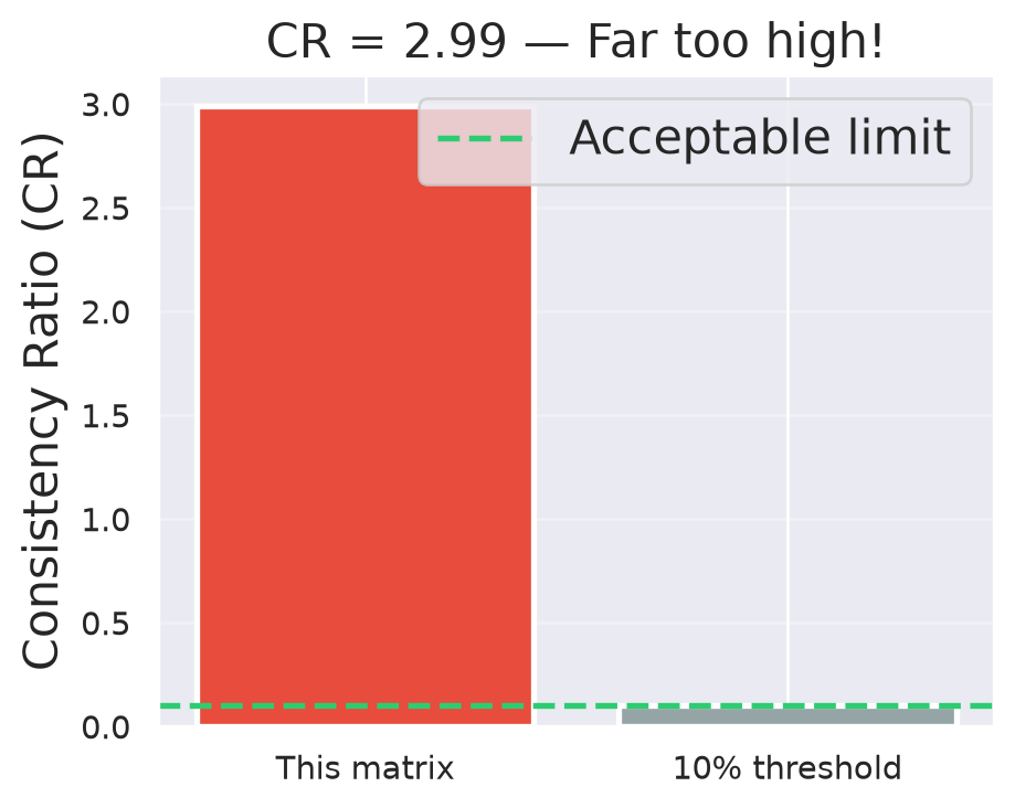
λ_max = 6.467, CI = 1.734, CR = 2.99

These judgments cannot be trusted — the planner needs to revisit them.

This example is designed to make inconsistency viscerally obvious. The planner’s judgments form a cycle: A dominates B, B dominates C, but C dominates A. This is like saying rock beats scissors, scissors beats paper, paper beats rock — there’s no coherent ranking.

The CR for this matrix will be very high (well above 0.10), which correctly flags the problem. The consistency check is not an arbitrary formality — it’s detecting that the judgment data is internally contradictory and would produce unreliable priorities.

Saaty (1990, p. 13) frames this precisely: “We now show the interesting, and perhaps surprising result that inconsistency throughout the matrix can be captured by a single number \(\lambda_{\max} - n\), which measures the deviation of the judgments from the consistent approximation.”

For a consistent matrix, \(\lambda_{\max} = n\) exactly. The greater the inconsistency, the larger \(\lambda_{\max}\) becomes. Theorem 1 proves \(\lambda_{\max} \geq n\) always, and Theorem 2 proves \(\lambda_{\max} = n\) if and only if the matrix is consistent.

How \(\lambda_{\max}\) Captures Inconsistency

The consistent case: The matrix has rank 1 (all information is redundant). Only one eigenvalue is nonzero, and it equals \(n\).

\[\lambda_{\max} = n, \quad \text{all other } \lambda_i = 0\]

. . .

The inconsistent case: The matrix has rank > 1. The “extra” information (contradictions) pushes \(\lambda_{\max}\) above \(n\).

\[\lambda_{\max} > n\]

. . .

The consistency index normalizes this deviation:

\[\text{CI} = \frac{\lambda_{\max} - n}{n - 1}\]

Why divide by \(n - 1\)?

A consistent matrix of order \(n\) has \(n - 1\) zero eigenvalues. When the matrix becomes inconsistent, these zeros become nonzero. The CI is their negative average.

. . .

Why compare to random matrices?

The RI tells us: “how inconsistent would a random set of judgments be?” If our CI is small relative to random noise, our inconsistency is acceptably low.

\[\text{CR} = \frac{\text{CI}}{\text{RI}} \leq 0.10\]

Saaty (1990, p. 13) proves two fundamental results:

Theorem 1. \(\lambda_{\max} \geq n\).

“Proof: Using \(a_{ji} = 1/a_{ji}\), and \(Aw = \lambda_{\max} w\), we have \(\lambda_{\max} - n = (1/n) \sum_{i<j} \delta_{ij}^2 / (1 + \delta_{ij}) \geq 0\)” where \(\delta_{ij}\) are the perturbations from perfect ratios.

Theorem 2. \(A\) is consistent if and only if \(\lambda_{\max} = n\).

“Proof. If \(A\) is consistent, then because of (1), each row of \(A\) is a constant multiple of a given row. This implies that the rank of \(A\) is one, and all but one of its eigenvalues \(\lambda_i\), \(i = 1, 2, \ldots, n\), are zero. However, it follows from our earlier argument that \(\sum_{i=1}^n \lambda_i = \text{Trace}(A) = n\). Therefore, \(\lambda_{\max} = n\).” (Saaty, 1990, p. 13)

The pedagogical approach here avoids requiring students to understand eigenvalue decomposition abstractly. Instead, the story is: 1. Consistent → all info is redundant → rank 1 → one eigenvalue = \(n\) 2. Inconsistent → contradictions introduce “extra dimensions” → rank > 1 → \(\lambda_{\max}\) grows 3. We measure how much it grew and compare to what random noise would produce

For the CI as a “negative average of the other eigenvalues”: since \(\sum \lambda_i = n\) always (trace is always \(n\) for a reciprocal matrix with 1’s on the diagonal), and the largest eigenvalue is \(\lambda_{\max}\), the remaining eigenvalues sum to \(n - \lambda_{\max}\). Their average is \((n - \lambda_{\max})/(n-1)\), which is the negative of CI.

Consistency: A Practical Summary

Random Index (RI) values and the 10% threshold

\(n\)	RI	Max acceptable CI
2	0.00	— (always consistent)
3	0.58	0.058
4	0.90	0.090
5	1.12	0.112
6	1.24	0.124
7	1.32	0.132
8	1.41	0.141

Why 10%?

Saaty (1990, p. 13): the threshold is “carefully specified to be about 10% or less.” It’s not a hard statistical cutoff — it’s a practical guideline calibrated against what random (i.e., meaningless) judgments would produce.

If CR > 0.10: revisit the most inconsistent judgment(s) and ask: “Do I really believe this?”

Saaty (1990, p. 13) explains: “For the consistency index (CI), we adopt the value \((\lambda_{\max} - n)/(n-1)\). It is the negative average of the other roots of the characteristic polynomial of \(A\). This value is compared with the same index obtained as an average over a large number of reciprocal matrices of the same order whose entries are random. If the ratio (called the consistency ratio CR) of CI to that from random matrices is significantly small (carefully specified to be about 10% or less), we accept the estimate of \(w\). Otherwise, we attempt to improve consistency.”

The RI values are obtained by generating many random reciprocal matrices and computing their average CI. A 2×2 reciprocal matrix is always consistent (there’s only one free parameter), so RI = 0. For larger matrices, random judgments produce increasing inconsistency.

Vargas (1982) “studied the case where the coefficients of the matrix are random variables. He focused his attention on gamma distributed coefficients and derived a Dirichlet distribution for the components of the eigenvector when the matrix is consistent. When the matrix is inconsistent, the 10% consistency bound is a sufficient measure to ensure that the eigenvector follows the Dirichlet distribution with given parameters.” (Saaty, 1990, p. 13–14)

The connection to Miller’s “magical number seven, plus or minus two” is also relevant: “He found that in general, people (such as chess experts) could deal with information involving simultaneously only a few facts, seven plus or minus two. […] This is in harmony with the stability of the principal eigenvalue to small perturbations when \(n\) is small.” (Saaty, 1990, p. 13)

VRP Example: Problem Setup

A logistics company has generated three candidate route plans for a daily delivery problem with 20 customers and 4 vehicles.

Metric	Plan A	Plan B	Plan C
Total distance (km)	142	158	135
Max driver hours	7.2	6.1	6.8
Workload std. dev. (h)	1.8	0.4	0.9

Plan profiles:

• Plan A: Short total distance, but one driver is overloaded
• Plan B: Longest distance, but very balanced workload
• Plan C: Moderate on both dimensions

Step 1: Structure the hierarchy (as shown earlier)

Step 2: Pairwise compare the criteria, then the alternatives under each criterion

This example is deliberately minimal — two criteria and three alternatives — to make the AHP mechanics transparent. In a real VRP setting, you might have 5–8 criteria (distance, number of vehicles, time window violations, driver balance, fuel cost, customer priority coverage, route compactness, etc.) and could be comparing dozens of candidate solutions generated by different metaheuristics or parameter settings.

Note that the raw data (km, hours) cannot simply be normalized and added. As Saaty warns, mixing scales requires care. The AHP sidesteps this entirely by working with pairwise judgments that produce ratio scales on a common basis.

Step 2a: Criteria Comparison

Question: For selecting the best route plan, how much more important is total distance vs. workload balance?

Suppose the planner judges distance to be moderately more important (3):

\[ C = \begin{pmatrix} 1 & 3 \\ 1/3 & 1 \end{pmatrix} \]

Priority vector (normalized eigenvector):

\[\mathbf{w}_C = \begin{pmatrix} 0.75 \\ 0.25 \end{pmatrix}\]

\(\lambda_{\max} = 2.000\), \(\text{CI} = 0.000\), \(\text{CR} = 0.000\) ✅

A \(2 \times 2\) reciprocal matrix is always perfectly consistent — there is only one free judgment.

For a 2×2 reciprocal matrix, consistency is guaranteed because there is only one independent judgment (the upper-right entry). The eigenvalue is always exactly \(n=2\).

The priority vector tells us the planner assigns 75% weight to total distance and 25% to workload balance. This is derived from the judgment, not assumed. If the planner had said “5” (strong importance), the weights would be approximately 83%/17%.

In the original house-buying example, Saaty used 8 criteria and found that “financing has the highest priority with 33% of the influence” (Saaty, 1990, p. 16). Our example is simpler but follows the same logic.

Step 2b: Alternatives vs. Distance

Question: Comparing route plans pairwise, how much better is one than another on total distance?

Recall: Plan A = 142 km, Plan B = 158 km, Plan C = 135 km.

\[ D = \begin{pmatrix} & A & B & C \\ A & 1 & 3 & 1/2 \\ B & 1/3 & 1 & 1/4 \\ C & 2 & 4 & 1 \end{pmatrix} \]

Priority vector: \(\mathbf{w}_D = (0.320,\; 0.122,\; 0.558)^T\)

\(\lambda_{\max} = 3.018\), \(\text{CI} = 0.009\), \(\text{CR} = 0.016\) ✅

The comparisons reflect that Plan C has the shortest distance (135 km), Plan A is close (142 km), and Plan B is the longest (158 km). The judgment that C is moderately better than A (value of 2 from C’s row perspective) and strongly better than B (value of 4) captures the planner’s assessment.

Note that we don’t mechanically convert the km values to ratios. As Saaty emphasizes, the pairwise comparison captures the decision-maker’s judgment about relative preference, which may incorporate nonlinear value functions. A difference of 7 km between C and A may be considered less significant than the difference of 23 km between C and B — the planner’s judgment of “2 vs. 4” reflects this.

The CR of 0.016 is well below the 0.10 threshold, indicating nearly perfect consistency. Let’s verify the transitivity: A vs B = 3, B vs C = 1/4, so A vs C should be 3 × 1/4 = 3/4. The actual judgment is 1/2, which is close but not exact — hence the small inconsistency.

Step 2c: Alternatives vs. Workload Balance

Question: Comparing route plans pairwise, how much better is one than another on workload balance?

Recall: Plan A std.dev. = 1.8h, Plan B std.dev. = 0.4h, Plan C std.dev. = 0.9h.

\[ W = \begin{pmatrix} & A & B & C \\ A & 1 & 1/7 & 1/3 \\ B & 7 & 1 & 3 \\ C & 3 & 1/3 & 1 \end{pmatrix} \]

Priority vector: \(\mathbf{w}_W = (0.072,\; 0.649,\; 0.279)^T\)

\(\lambda_{\max} = 3.007\), \(\text{CI} = 0.003\), \(\text{CR} = 0.006\) ✅

Here the comparisons reflect that Plan B has by far the best workload balance (std. dev. of only 0.4h), Plan C is moderate (0.9h), and Plan A is poor (1.8h). The judgment of 7 (very strong importance of B over A) captures the substantial difference in balance.

Again, the CR is very low (0.006), indicating highly consistent judgments. In practice, when the decision-maker has concrete data to inform the pairwise comparisons, consistency tends to be high. Inconsistency becomes more of an issue when judgments are purely subjective.

Step 3: Global Priorities

Combine local priorities using the criteria weights:

\[ \text{Global priority}_i = \sum_{j} w_{C_j} \cdot w_{ij} \]

	Distance (0.75)	Balance (0.25)	Global
Plan A	0.320	0.072	0.258
Plan B	0.122	0.649	0.254
Plan C	0.558	0.279	0.488

Result

Plan C is the recommended choice with 48.8% of the overall priority, followed closely by Plan A (25.8%) and Plan B (25.4%).

Following Saaty’s procedure: “We lay out the local priorities of the [alternatives] with respect to each criterion in a matrix and multiply each column of vectors by the priority of the corresponding criterion and add across each row which results in the desired vector.” (Saaty, 1990, p. 17)

The computation for Plan C: \(0.75 \times 0.558 + 0.25 \times 0.279 = 0.419 + 0.070 = 0.488\).

Interestingly, Plan C wins despite not being the best on either individual criterion — it is a strong compromise. Plan A has the second-best distance but poor balance; Plan B has excellent balance but poor distance. This mirrors Saaty’s house-buying example where “House A which was the least desirable with respect to financing (the highest priority criterion), contrary to expectation, had the largest priority.” (Saaty, 1990, p. 17)

This illustrates a key strength of the AHP: it can identify compromise solutions that would not be obvious from looking at individual metrics.

Sensitivity: What If Balance Matters More?

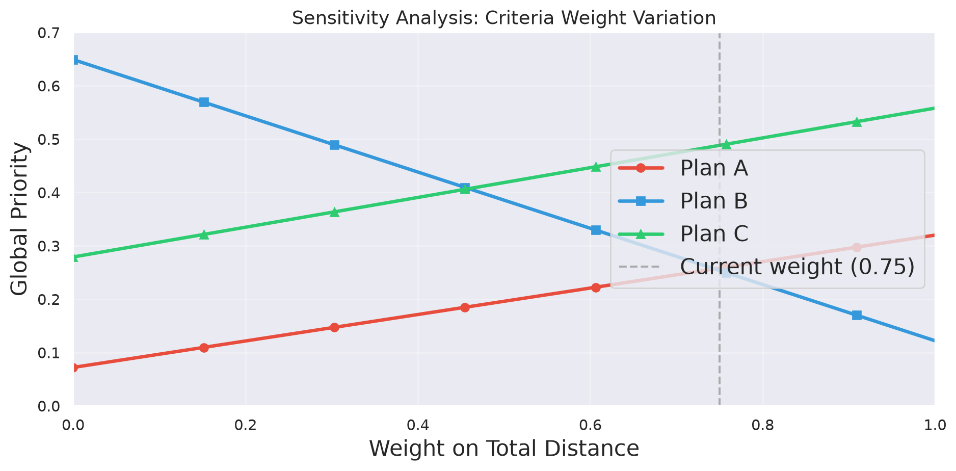
Let’s vary the criteria weight for distance from 0 to 1:

Sensitivity analysis is a critical step in AHP applications. The chart shows how the global priorities change as we vary the weight on total distance.

Key observations:

• Plan C dominates across a wide range of criteria weights (roughly from 0.35 to 1.0).
• Plan B becomes the best choice only when the weight on distance drops below about 0.35 — meaning the planner cares primarily about workload balance.
• Plan A is never the top-ranked alternative for any weight combination, because Plan C dominates it on distance and Plan B dominates it on balance.

This kind of analysis is supported by software like Expert Choice, which Saaty mentions: “The software package Expert Choice, useful in teaching and in real applications, can handle both relative and absolute measurement, as well as having special capabilities such as structural rescaling, combining group judgments, sensitivity analysis and dependence among the decision alternatives.” (Saaty, 1990, p. 20)

Scarcity and Abundance in VRP

Saaty introduces a nuanced idea about how criteria differentiate alternatives:

• A criterion where all plans score similarly is “abundant” — it contributes little to rank determination
• A criterion where plans differ sharply is “scarce” — it is decisive

In our example:

Criterion	Contrast	Effect
Distance	Moderate	Moderate influence
Balance	High	High influence per unit weight

This means even a lower-weighted criterion can be decisive if it provides high contrast among alternatives.

Saaty (1990, p. 20) explains: “Normalization can also be associated with the idea of scarcity and abundance of the presence of a criterion in the alternatives. […] Thus, the greater the contrast among the alternatives, the more useful is the priority value of the criterion allotted to each.”

He formalizes this: “An ‘abundant’ criterion contributes less to rank determination because it contributes an equal or nearly equal priority to each alternative and when the sum is taken over the criteria it has little effect in determining rank.” (p. 20)

Theorem 4 in the paper states that \(\sum_{ij} a_{ij} = n^2\) if and only if all alternatives have equal dominance (\(a_{ij} = 1\) for all \(i,j\)). So \(n^2\) is the minimum total dominance, corresponding to zero discriminating power.

In VRP terms: if you have 10 candidate route plans that are all within 1% of each other on total distance but vary wildly on workload balance, then balance effectively becomes the deciding factor even if it has a lower weight.

Relative vs. Absolute Measurement

Saaty describes two modes of AHP:

Relative Measurement

• Compare alternatives pairwise under each criterion
• Best for small sets of distinct alternatives
• Rank can change when alternatives are added/removed

VRP use: Comparing 3–5 candidate route plans from different solvers.

Absolute Measurement (Ratings)

• Define grade levels per criterion (e.g., Excellent, Good, Average, Poor)
• Rate each alternative against these standards
• Rank is preserved when alternatives are added/removed

VRP use: Rating 100+ route plans against predefined quality standards.

Saaty (1990, p. 14) explains: “In relative measurement, paired comparisons are performed throughout the hierarchy including on the alternatives. […] In absolute measurement, paired comparisons are also performed through the hierarchy with the exceptions of the alternatives themselves.”

For absolute measurement, he describes: “The level just above the alternatives consists of intensities or grades which are refinements of the criteria or subcriteria governing the alternatives. […] The alternatives are not pairwise compared, but simply rated as to what category in which they fall under each criterion.” (p. 14)

In a VRP context, absolute measurement is particularly useful when a fleet manager needs to evaluate many route plans against company standards. For example, a route plan could be rated as “Excellent” on distance if it’s within 5% of the lower bound, “Good” if within 10%, etc.

Saaty notes: “There is no reason why forcing standards on a problem should produce the same outcome obtained through relative measurement. These are two different descriptive (what can be) and normative (what should be) settings.” (p. 14)

Practical Considerations

Strengths for VRP

• Transparent weighting of KPIs
• Handles intangible criteria (driver satisfaction, route aesthetics)
• Built-in consistency check
• Supports group decision making (combine planners’ judgments)

Limitations

• Number of pairwise comparisons grows as \(n(n-1)/2\)
• Assumes hierarchical independence of criteria
• Potential rank reversal in relative mode when alternatives change
• Subjectivity in pairwise judgments

For large VRP instances

Use absolute measurement with predefined quality grades, or cluster alternatives before relative comparison (Saaty, Section 7).

The clustering section of Saaty’s paper (Section 7, p. 20-21) is particularly relevant for VRP where we may have many candidate solutions. He describes three approaches: the elementary approach (highly inefficient, requiring \((n-1)!\) comparisons), trial-and-error clustering, and clustering by absolute measurement.

For VRP, the recommendation is: “For many problems, it is useful to first carry out absolute measurement to sort and cluster the elements, and then follow that with relative measurement for greater accuracy.” (Saaty, 1990, p. 21)

On rank reversal, Saaty (1990, p. 25) notes: “The absolute mode of measurement of the AHP complies with this normative inclination [preserving rank], but the relative mode of measurement does not, because of the dependence of the measurements of the alternatives on each other.”

Summary

The AHP provides:

1. A structured framework for balancing competing VRP objectives
2. Ratio scales derived from pairwise judgments — not arbitrary scores
3. The eigenvector as the natural method for extracting weights from all direct and indirect comparisons
4. A consistency check rooted in how far \(\lambda_{\max}\) deviates from \(n\)
5. Sensitivity analysis to understand robustness

Key takeaway for VRP:

When choosing among route plans, the “best” depends on how you weight the criteria. AHP makes this weighting explicit, traceable, and mathematically grounded.

Reference

Saaty, T.L. (1990). How to make a decision: The Analytic Hierarchy Process. European Journal of Operational Research, 48(1), 9–26. doi:10.1016/0377-2217(90)90057-I

Saaty (1990, p. 25–26) summarizes: “The AHP generates relative ratio scales of measurement. The measurements of a set of objects on a standard scale can be converted to relative scale measurements through normalization.”

His closing thought is worth reflecting on: “We believe that our own tempered understanding should produce closer results to experience than simply following tradition, which has possibly rutted our thinking, and induced us to forego change in search of better ways that give better answers.” (Saaty, 1990, p. 26)

For further reading: - Saaty’s book Multicriteria Decision Making: The Analytic Hierarchy Process (1980/1988) provides the full treatment. - Vargas (1990) in the same EJOR issue provides an applications overview. - Zahedi (1986) in Interfaces surveys the method and its applications. - For VRP-specific multicriteria approaches, see Jozefowiez et al. (2008) in EJOR for a survey of multi-objective VRP.

Appendix: Computing Eigenvectors

For small matrices, the eigenvector can be approximated by repeated squaring and normalization:

Priority vector: [0.75 0.25]
λ_max = 2.000, CI = 0.000

Saaty (1990, p. 19) describes the computational procedure: “The solution of the eigenvalue problem is obtained by raising the matrix \(A\) to a sufficiently large power then summing over the rows and normalizing to obtain the priority vector \(w = (w_1, \ldots, w_n)^T\). The process is stopped when the difference between components of the priority vector obtained at the \(k\)-th power and at the \((k+1)\)st power is less than some predetermined small value.”

The power method shown here is the simplest implementation. Students can also verify with numpy’s linalg.eig function. The key point is that raising the matrix to successive powers and normalizing the row sums is exactly the “dominance walk” computation from Theorem 3 — so the computation directly mirrors the conceptual justification.

Saaty, Thomas L. 1990. “How to Make a Decision: The Analytic Hierarchy Process.” European Journal of Operational Research 48 (1): 9–26. https://doi.org/10.1016/0377-2217(90)90057-I.