Multi-Objective Optimization

Concepts and solution techniques

Eduardo Lalla-Ruiz

University of Twente

Date

2026-08-14

Models, shortest paths, routing, piecewise linearization, and multi-objective optimization.

What is a Mathematical Model?

Lecture

Introduction to modeling in mathematical optimization

01

In the famous painting The School of Athens by Raphael, Plato is shown pointing up (to the heavens) and Aristotle is pointing down (to the earth). This perfectly captures their disagreement. Plato believed in ideal forms that exist in a perfect realm, while Aristotle focused on the tangible world around us. In optimization modeling, we often create idealized mathematical representations of real-world problems. These models are not perfect replicas of reality, but they capture essential features to help us understand and solve complex issues. Just like Plato’s forms, our models are abstractions that allow us to reason about the world in a structured way.

In aristotelian terms, a mathematical model is a “form” that captures the “essence” of a problem. It abstracts away irrelevant details while retaining the core structure needed for analysis and optimization. This lecture will introduce the concept of mathematical models in the context of logistics optimization, setting the stage for more complex formulations in later lectures.

Plato’s idealism vs. Aristotle’s realism is a useful lens for understanding the role of models: they are not perfect representations of reality, but tools that help us navigate and optimize within it.

What Is a Model?

A model is…

…a structure built to exhibit features and characteristics of some other objects. Generally, only some of these features and characteristics will be retained in the model depending upon the use to which it is to be put. — (Williams 2013)

A model allows us to study a system and its components, providing solutions and predictions about its behavior.

1.1 The concept of a model.

Many applications of science make use of models. The term ‘model’ is usually used for a structure built to exhibit features and characteristics of some other objects. Generally, only some of these features and characteristics will be retained in the model depending upon the use to which it is to be put.

Sometimes such models are concrete, as with a model aircraft used in wind-tunnel experiments. More often in operational research we deal with abstract models, usually mathematical, where algebraic symbolism mirrors the internal relationships of the object being modelled. Our attention here is mainly confined to such mathematical models, though ‘model’ is sometimes used more widely to include purely descriptive models.

Are All Models Wrong?

In strict sense, yes.

A map is not the territory. — Alfred Korzybski

However, the value of a model lies in its usefulness for understanding, decision-making, and problem-solving, not in its perfect accuracy. Therefore:

All models are wrong, but some are useful. — George Box

A good model captures the essential features of a problem while ignoring irrelevant details. Still, be critical.

Trust, but verify. — Ronald Reagan

There is no reason to trust a model without scrutiny. Always question the assumptions, data, and outputs of a model to ensure it is providing reliable insights for decision-making.

Misconceptions about the value of mathematical models exist. At one extreme, some deny models have any value for planning, often citing the difficulty of quantifying required data (for example, attaching a cost or utility to a social value). A less severe criticism concerns the lack of precision in much model data; if many coefficients are uncertain, confidence in produced answers may be low. The first criticism is difficult to counter; making implicit quantifications explicit in a mathematical model can be more honest and scientific. The second criticism should be assessed per model: even with inaccurate coefficients, the model’s structure may produce little inaccuracy in the solution.

At the opposite extreme are those who place almost metaphysical faith in a mathematical model for decision making. The quality of answers depends on the accuracy of the model structure and data; uncritical faith is unwarranted and dangerous. Accepting the first answer from a model without further analysis should be rare. A model should be used as one of several decision-making tools. Model outputs should be scrutinized; if unacceptable, reasons should be identified and, if possible, incorporated into a modified model. Specifying another objective function may produce a different option. By successive questioning and altering the model (or its objective), one can clarify available options and achieve a greater understanding of what is possible. (Williams 2013, 3)

What is a Mathematical Model?

A mathematical model is…

… a set of mathematical relationships (equations, inequalities, logical dependencies) that correspond to more down-to-earth relationships in the real world (technological relationships, physical laws, marketing constraints). — (Williams 2013)

The essential feature of a mathematical model in operational research is that it involves a set of mathematical relationships (equations, inequalities, logical dependencies) that correspond to more down-to-earth relationships in the real world (technological relationships, physical laws, marketing constraints).

Why Build a Mathematical Model?

According to Williams (2013), there are three main reasons for building mathematical models:

1. Constructing a model often uncovers hidden relationships and deepens understanding of the system.
2. Once formulated, a model can be analyzed mathematically to reveal actionable options not otherwise evident.
3. A model allows controlled experimentation that would be impractical, unsafe, or impossible on the real system.

There are a number of motives for building such models: 1. The exercise of building a model often reveals relationships not previously apparent, yielding greater understanding of the object being modelled. 2. Once built, a model can often be analysed mathematically to suggest courses of action that might not otherwise be apparent. 3. Experimentation is possible with a model, whereas it is often not possible or desirable to experiment with the real object.

A model is really defined by the relationships it incorporates. These relationships are largely independent of the data in the model. A model may be reused with differing data (costs, technological coefficients, resource availabilities) and still be regarded as the same model. Radical changes in data, however, may imply changes in the relationships and so a different model.

Mathematical Programming Models

• In Operations Research (OR), models are formulated using standard forms, among which mathematical programming¹ is the most common.
• There are many classes of mathematical programming, including:
  • Linear programming (LP). Models with linear relationships.
  • Nonlinear programming (NLP). Models with nonlinear relationships.
  • Integer programming (IP).² Models where some or all decision variables are constrained to take integer values.

Many models in operational research take standard forms. The mathematical-programming type is a commonly used standard form. Other examples include simulation models, network planning models, econometric models and time-series models. This list is not exhaustive; practical situations sometimes require non-standard models. Comparing results from different model types can be extremely valuable.

Mathematical programming vs computer programming

Mathematical programming is ‘programming’ in the sense of ‘planning’, not computer programming. As planning, it need have nothing to do with computers. However, practical problems typically require large amounts of data and arithmetic that are most reasonably handled by computers.

1. “Programming” in mathematical programming refers to “planning” rather than computer programming. While computers are often used to solve these models, the term emphasizes the structured approach to decision-making rather than coding.

2. Mixed-integer programming (MIP) and mixed-integer linear programming (MILP) are subcategories of integer programming where only some decision variables are required to be integers, while others can be continuous.

The Anatomy of a Mathematical Programming Model

A common structure of mathematical programming models includes four key components (see Figure 1).

graph TD
    P["<b>Parameters</b><br>Given data that<br>does not change"] --> M["Mathematical<br>Model"]
    V["<b>Decision Variables</b><br>What we control<br>and optimize"] --> M
    C["<b>Constraints</b><br>Limitations on<br>feasible solutions"] --> M
    O["<b>Objective Function</b><br>KPI to maximize<br>or minimize"] --> M

Figure 1: The four core components of any optimization model.

A common feature of mathematical programming models is that they involve optimization. We wish to maximize or minimize a quantity known as the objective function. The focus on an objective sometimes leads to the mistaken belief that mathematical programming is unusable when no clear objective exists or when multiple objectives are present. Often, optimizing some aspect of a model remains useful even in such cases.

This text concentrates on three classes of mathematical programming: linear programming (LP), nonlinear programming (NLP), and integer programming (IP). We begin by describing LP models through two small examples. (Williams 2013, 5)

Example: A Mobility Company Route Optimization Problem

• Problem Statement. A mobility company needs to design routes for a fleet of vehicles to pick up and deliver passengers.

• Objective Function(s). Minimize total travel time, minimize total distance, maximize customer satisfaction, etc.

• Decisions. Which vehicle serves which passenger, and in what order? When do vehicles arrive at pickup and drop-off locations? Where do vehicles start and end their routes?

• Constraints. Each passenger must be picked up and dropped off within their time windows. Vehicle capacity limits must not be exceeded. Each vehicle route must start and end at the depot.

• Parameters. Travel times between locations, passenger demand (pickup/drop-off locations and time windows), vehicle capacities, fleet size, depot location, etc.

The Modeling Framework

Figure 2 illustrates the general workflow for mathematical modeling in optimization.

graph LR
    A(("Real World<br><b>Problem</b>")) --> S[/"Quantitative &<br>Qualitative Data"/]
    S --> B["Model Construction<br><b>Parameters, Variables,</b><br><b>Constraints, Objective</b>"]
    B --> C["Model Solution<br><b>Solver / Algorithm</b>"]
    C --> D["Conclusions<br><b>Interpret Results</b>"]
    D --> E{"Valid?"}
    E -- "Yes" --> F[/"Solution to<br>Real-World Problem"/]
    E -- "No" --> B

Figure 2: The mathematical modeling workflow: from real world to validated solution.

Data collection: quantitative data (numbers, measurements) and qualitative data (interviews, observations). If validation fails, iterate back to model construction.

Conclusion

• A mathematical model is a structured representation of a real-world problem using mathematical relationships.
• Models are simplifications of reality, but they can provide valuable insights and solutions when used critically.
• The core components of a mathematical programming model include parameters, decision variables, constraints, and an objective function.
• The modeling process involves iterating between understanding the real-world problem, constructing a model, solving it, and validating the results against reality.

References

Ahuja, Ravindra K., Thomas L. Magnanti, and James B. Orlin. 1993. Network Flows: Theory, Algorithms, and Applications. Prentice Hall.

Arora, Jasbir S. 2017. “Multi-Objective Optimum Design Concepts and Methods.” In Introduction to Optimum Design, 4th ed. Elsevier. https://doi.org/10.1016/B978-0-12-800806-5.00018-4.

Boeing, Geoff. 2017. “OSMnx: New Methods for Acquiring, Constructing, Analyzing, and Visualizing Complex Street Networks.” Computers, Environment and Urban Systems 65: 126–39. https://doi.org/10.1016/j.compenvurbsys.2017.05.004.

Brown, Gerald G., and Robert F. Dell. 2007. “Formulating Integer Linear Programs: A Rogues’ Gallery.” INFORMS Transactions on Education 7 (2): 153–59.

Caramia, Massimiliano, and Paolo Dell’Olmo. 2008. Multi-Objective Management in Freight Logistics. Springer.

Chang, Kuang-Hua. 2015. “Multiobjective Optimization and Advanced Topics.” In Design Theory and Methods Using CAD/CAE. Elsevier. https://doi.org/10.1016/B978-0-12-398512-5.00005-0.

Chankong, Vira, and Yacov Y. Haimes. 1983. Multiobjective Decision Making: Theory and Methodology. Elsevier.

Clarke, G., and J. W. Wright. 1964. “Scheduling of Vehicles from a Central Depot to a Number of Delivery Points.” Operations Research 12 (4): 568–81.

Croxton, Keely L., Bernard Gendron, and Thomas L. Magnanti. 2003. “A Comparison of Mixed-Integer Programming Models for Nonconvex Piecewise Linear Cost Minimization Problems.” Management Science 49 (9): 1268–73. https://doi.org/10.1287/mnsc.49.9.1268.16570.

Dantzig, George B., and John H. Ramser. 1959a. “The Truck Dispatching Problem.” Management Science 6 (1): 80–91.

Dantzig, George B., and John H. Ramser. 1959b. “The Truck Dispatching Problem.” Management Science 6 (1): 80–91.

DHL Express. 2026. Service & Rate Guide 2026: Netherlands. PDF. https://www.dhlexpress.nl/sites/default/files/content/Netherlands%20English%20SARG26%20Full%20DEF.pdf.

Dijkstra, Edsger W. 1959. “A Note on Two Problems in Connexion with Graphs.” Numerische Mathematik 1: 269–71.

FedEx. 2026. Information on Your Rates and Shipments: Applicable in the Netherlands from 5 January 2026. PDF. https://www.fedex.com/content/dam/fedex/international/rates/new-offer-rates-domestic-en-nl.pdf.

Gendreau, Michel, Alain Hertz, and Gilbert Laporte. 1994. “A Tabu Search Heuristic for the Vehicle Routing Problem.” Management Science 40 (10): 1276–90.

Geoffrion, Arthur M. 1968. “Proper Efficiency and the Theory of Vector Maximization.” Journal of Mathematical Analysis and Applications 22 (3): 618–30.

Golden, Bruce L., Arjang A. Assad, Leon Levy, and Frederic G. Gheysens. 1984. “The Fleet Size and Mix Vehicle Routing Problem.” Computers & Operations Research 11 (1): 49–66.

Hitchcock, Frank L. 1941. “The Distribution of a Product from Several Sources to Numerous Localities.” Journal of Mathematics and Physics 20 (1-4): 224–30.

Lalla-Ruiz, Eduardo, and Stefan Voß. 2020. “A POPMUSIC Approach for the Multi-Depot Cumulative Capacitated Vehicle Routing Problem.” Optimization Letters 14 (3): 671–91.

Maffioli, Federico, and Anna Sciomachen. 2015. Chapter 2: Multi-Objective Optimization. PDF.

Miettinen, Kaisa. 1994. On the Methodology of Multiobjective Optimization with Applications. University of Jyväskylä.

Miller, Clair E., Albert W. Tucker, and Richard A. Zemlin. 1960. “Integer Programming Formulation of Traveling Salesman Problems.” Journal of the ACM 7 (4): 326–29.

Montoya-Torres, Jairo R., Julián López Franco, Santiago Nieto Isaza, Heriberto Felizzola Jiménez, and Nilson Herazo-Padilla. 2015. “A Literature Review on the Vehicle Routing Problem with Multiple Depots.” Computers & Industrial Engineering 79: 115–29.

Munson, Charles L., and Meir J. Rosenblatt. 1998. “Theories and Realities of Quantity Discounts: An Exploratory Study.” Production and Operations Management 7 (4): 352–69. https://doi.org/10.1111/j.1937-5956.1998.tb00127.x.

Murray, Chase C., and Amanda G. Chu. 2015. “The Flying Sidekick Traveling Salesman Problem: Optimization of Drone-Assisted Parcel Delivery.” Transportation Research Part C: Emerging Technologies 54: 86–109.

National Motor Freight Traffic Association. 2026. Freight Classification Development Council Procedures 2026. PDF. https://nmfta.org/wp-content/media/2026/01/FCDC-Procedures-2026.pdf.

OpenStreetMap Foundation. 2026. “OpenStreetMap Copyright and License.” https://www.openstreetmap.org/copyright.

Psaraftis, Harilaos N. 1980. “A Dynamic Programming Solution to the Single Vehicle Many-to-Many Immediate Request Dial-a-Ride Problem.” Transportation Science 14 (2): 130–54.

Solomon, Marius M. 1987a. “Algorithms for the Vehicle Routing and Scheduling Problems with Time Window Constraints.” Operations Research 35 (2): 254–65.

Solomon, Marius M. 1987b. “Algorithms for the Vehicle Routing and Scheduling Problems with Time Window Constraints.” Operations Research 35 (2): 254–65.

Sudhoff, Scott. 2007. Lecture 9: Multi-Objective Optimization. PDF slides.

Williams, Paul. 2013. Model Building in Mathematical Programming. 5th ed. Wiley.

Mathematical Model Components

Lecture

Parameters, decision variables, objective function, and constraints

02

Introduction

Mathematical models comprise the following key components:

• Parameters: the given information that defines the problem context.
• Decision variables: the unknowns that represent the choices to be made.
• Constraints: the limitations and requirements that must be satisfied.
• Objective function: the KPI to optimize (minimize or maximize).

Parameters (Data / Input)

Parameters are the given information that remains fixed for a problem instance.

• They are coefficients in the model that quantify the problem context, such as costs, capacities, demands, distances, time windows, etc.
• They are often organized in arrays or indexed structures to represent relationships between entities.

Decisions

First, what is a decision?

As put by Prof. Warren Powell, a decision is:

Something we control.

Therefore:

If you want to run a better \(\left\{\begin{array}{lllll}\text{Supply chain} & \text{Energy system} & \text{Transportation network} & \text{Healthcare operations} & \text{Manufacturing process}\end{array}\right\}\) you have to make better decisions.

Decision Variables

Decision variables represent the choices the model can make.

• They are the unknowns that the optimization process will solve for, and they determine the solution to the problem.
• Types of decision variables include:
  • Continuous: can take any non-negative fractional value (e.g., quantity shipped).
  • Binary: can only be 0 or 1 (e.g., whether to open a facility).
  • Integer: can take whole number values (e.g., number of vehicles used).

Decision Variable Notation

In math programming, a decision variable is often denoted as \(x\), \(y\), or \(z\), with subscripts or superscripts to indicate its specific role. For example:

• \(x_{ij}\) might represent the quantity shipped from location \(i\) to location \(j\).
• \(x_{ij}^k\) could indicate which vehicle \(k\) is assigned to route from \(i\) to \(j\).
• \(y_i\) could indicate whether a customer \(i\) is served (1) or not (0).
• \(z_k\) might represent the number of vehicles of type \(k\) used in a routing problem.

Modeling Tip: Upright labels in math

Use upright text for multi-letter labels in subscripts/superscripts to avoid ambiguity. Use \text{...} for words; use \mathrm{...} for abbreviations.

Bad: \(x_{job}\) (ambiguous, are \(j\), \(o\), and \(b\) separate variables?)

Good: - \(x_{\text{job}}\) (word label). - \(x_{\mathrm{NY}}\) (abbreviation). - \(x_{i,j}\) (indices). - \(x_{i,\text{job}}\) (index + label).

Keep the style consistent across the model.

Objective Function

The objective defines what to optimize — either maximize or minimize a given KPI.

• It must be carefully defined to reflect the true goals of the problem, as optimizing the wrong objective can lead to suboptimal or even harmful decisions.
• Multiple objectives can be combined into a single objective using weighted sums or handled separately in multi-objective optimization frameworks.

Linearity Requirement

Although some optimization problems can be nonlinear, in integer linear programming (ILP) the objective function must be linear. This means you cannot have products of decision variables in the objective without applying a linearization technique.

Be Aware of the Cobra Effect

Choosing the wrong key performance indicators (KPIs) for the objective function can lead to unintended consequences, a phenomenon known as the “Cobra Effect.”

“The Cobra Effect” is a cautionary tale: the British colonial government (allegedly) paid bounties for dead cobras, leading people to breed them for profit. When the program ended, breeders released the snakes, and the population increased.

Picking a certain KPI can deteoriate many others. Commonly:

There are no solutions, only trade-offs. — Thomas Sowell

The Cobra Effect is a phenomenon where an intended solution to a problem actually makes the problem worse. It is named after a historical incident in colonial India, where the British government offered a bounty for dead cobras in an attempt to reduce the cobra population. However, instead of decreasing the cobra population, this policy led to an increase in cobra breeding, as people started to breed cobras in order to collect the bounty.

The Cobra Effect is a common occurrence in public policy and management, where well-intentioned solutions backfire because they fail to take into account the incentives and motivations of the people affected by the policy. One example of the cobra effect is when governments offer subsidies for certain products, it can lead to overproduction of those products, which can then lead to an oversupply and prices drop.

Another example of the Cobra effect can be seen in the context of performance metrics. When a manager sets a target for their team, and the team focuses on achieving that target, they may neglect other important aspects of their job, or even engage in unethical behavior to meet the target.

Example: Trade-offs in the Pickup and Delivery Problem (PDP)

In the Pickup and Delivery Problem (PDP), we have a set of vehicles, customers with pickup and delivery locations, and we need to determine the routes for the vehicles to serve the customers. Depending on the objective function we choose, we can end up with very different optimal routes. Figure 38 illustrates a simple PDP scenario.

We will consider the following objectives:

• Minimize fleet size (number of vehicles used)
• Minimize pickup waiting time (time between pickup request and pickup)

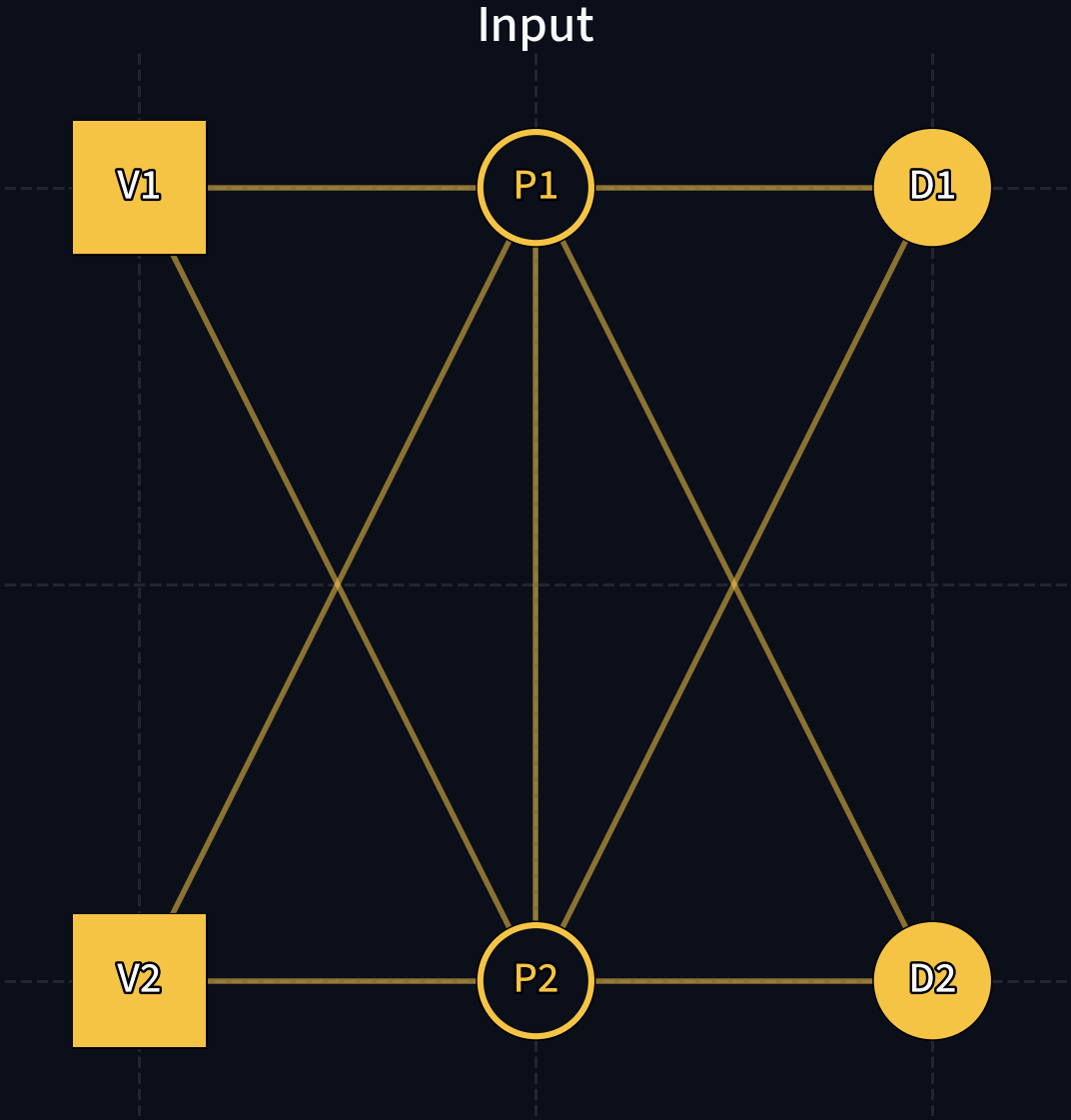
Figure 3: Input scenario: Two vehicles (V1, V2), two pickups (P1, P2), and two dropoffs (D1, D2). For simplicity, all distances are unitary (time and distance).

Input scenario only. This map is repeated in the panel for direct comparison against routes R1–R5.

Trade-offs: Fleet Utilization vs. Service Level

1. If we minimize total distance, we get a single route (see Figure 4). However, P1 or P2 will have to wait 1 unit of time more.
2. If we minimize pickup waiting time, we get two routes (see Figure 40). However, this requires using two vehicles instead of one.

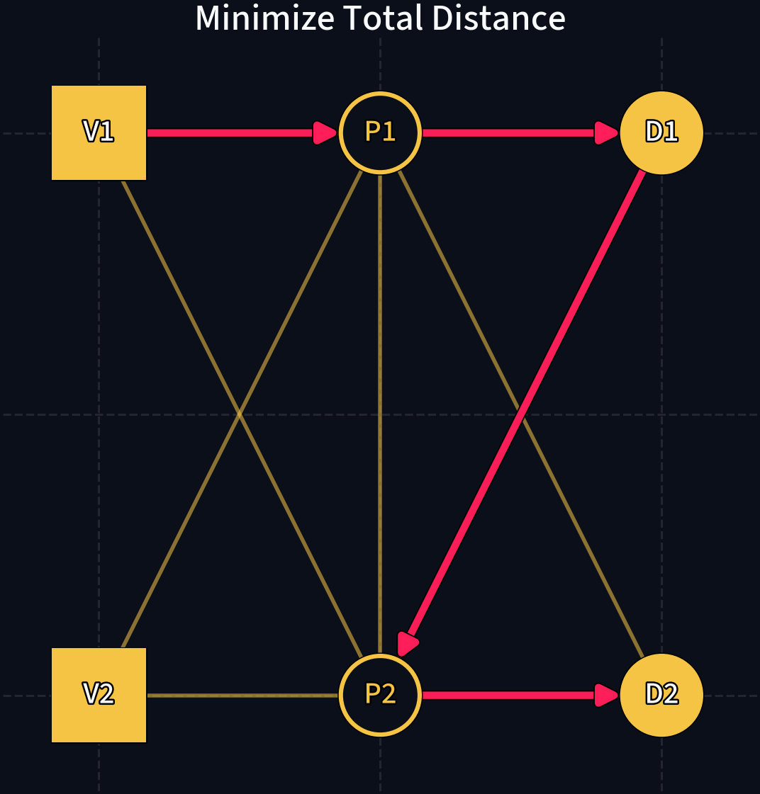
Figure 4: Minimizing distance leads to a single-vehicle route: V1->P1->P2->D2->P1->D1.

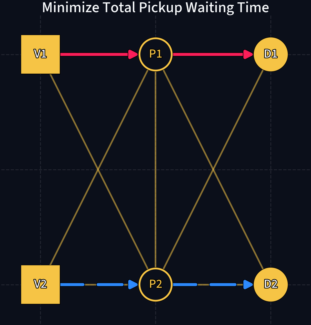
Figure 5: Minimizing pickup waiting time leads to two routes: V1->P1->D1 and V2->P2->D2.

Constraints

Constraints express the limitations of the problem. For example:

• A factory can produce at most 100 units per day (capacity constraint).
• A customer must receive at least 50 units (demand constraint).
• A service cannot reject more than 10% of its demand (service level constraint).
• Working shifts must be assigned to employees without overlap (scheduling constraint).
• A vehicle cannot exceed its load capacity (weight constraint).
• A route must start and end at the depot (routing constraint).

Linearity Requirement

In integer linear programs, constraints must be linear — you cannot multiply two decision variables together without applying a linearization technique.

Transportation Problem

Lecture

Basics and formulation

03

Section divider: introduce classical TP and its uses.

Problem Statement

From the seminal work by Hitchcock (1941):

When several factories supply a product to a number of cities, we desire the least costly manner of distribution. Due to freight rates and other matters, the cost of a ton of product to a particular city will vary according to which factory supplies it, and will also vary from city to city.

Model Notation

Sets and indices:

• \(M\) = set of factories (supply nodes)
• \(N\) = set of cities (demand nodes)
• \(i \in M\) = factory index
• \(j \in N\) = city index

Parameters:

• \(a_i\) = capacity of factory \(i\)
• \(b_j\) = demand of city \(j\)
• \(c_{ij}\) = cost per unit from \(i\) to \(j\)

Decision variable:

• \(x_{ij} \in \mathbb{R}_{\geq 0}\) = units sent from \(i\) to \(j\)

Model Formulation

Objective: Minimize total transportation cost.

Constraints:

• Supply limits at factories (Equation 1)
• Demand requirements at cities (Equation 2)
• Nonnegativity of shipments (Equation 3)

Balanced Case

When \(\sum_i a_i = \sum_j b_j\), the supply constraints can use \(=\) instead of \(\leq\), and demand constraints can also use \(=\).

LP Formulation: \[ \min \sum_{i \in M} \sum_{j \in N} c_{ij} x_{ij} \]

subject to: \[ \sum_{j \in N} x_{ij} \leq a_i \quad \forall \, i \in M \quad \text{(supply)} \tag{1}\]

\[ \sum_{i \in M} x_{ij} \geq b_j \quad \forall \, j \in N \quad \text{(demand)} \tag{2}\]

\[ x_{ij} \geq 0 \quad \forall \, i \in M, \, j \in N \quad \text{(nonnegativity)} \tag{3}\]

Example: 3 Factories, 4 Cities

A transportation company aims to minimize total transportation costs from 3 factories (\(S_1, S_2, S_3\)) to 4 cities (\(D_1, D_2, D_3, D_4\)), given factory capacities and city demands (see Figure 6).

graph LR
    subgraph "Factories (Supply)"
        S1["S1<br>$a_1$ units"]
        S2["S2<br>$a_2$ units"]
        S3["S3<br>$a_3$ units"]
    end
    subgraph "Cities (Demand)"
        D1(("D1<br>$b_1$ units"))
        D2(("D2<br>$b_2$ units"))
        D3(("D3<br>$b_3$ units"))
        D4(("D4<br>$b_4$ units"))
    end
    S1 -- "$c_{11}$" --> D1
    S1 -- "$c_{12}$" --> D2
    S2 -- "$c_{23}$" --> D3
    S3 -- "$c_{34}$" --> D4

Figure 6: Bipartite network: factories supply cities at varying costs per unit. Each edge’s label \(c_{ij}\) represents the cost per unit from factory \(i\) to city \(j\). The company must determine how many units \(x_{ij}\) to ship along each route to satisfy demand.

Model Formulation

Using data from Table 1, Table 2, and Table 3, we can build the model:

\[\begin{aligned} \min \quad & 2x_{11} + 6x_{12} + 5x_{21} + 3x_{22} \\ \text{subject to} \quad & x_{11} + x_{12} \leq 5 \quad \text{(S1 supply)} \\ & x_{21} + x_{22} \leq 3 \quad \text{(S2 supply)} \\ & x_{11} + x_{21} \geq 4 \quad \text{(D1 demand)} \\ & x_{12} + x_{22} \geq 4 \quad \text{(D2 demand)} \\ & x_{ij} \geq 0 \quad \forall i, j \end{aligned}\]

Parameters

Upon gathering data, for the instance presented in Figure 6, we have the factory capacities (Table 1), city demands (Table 2), and unit costs (Table 3).

Table 1: Factory capacities.

Factory \(i\)	Supply \(a_i\)
S1	5
S2	3

Table 2: City demands.

City \(j\)	Demand \(b_j\)
D1	4
D2	4

Table 3: Unit shipping costs \(c_{ij}\).

\(c_{ij}\)	D1	D2
S1	2	6
S2	5	3

Avoid Data Collection Paralysis

Note that the model can be formulated (and implemented, see Listing 3) independently of the specific data values. In practice, data collection can be a bottleneck, but the model structure can be defined first and data can be filled in iteratively.

Solution: Using an LP Solver

Using PuLP, a free linear programming library in Python, we can model (see Listing 1) and solve (see Listing 2) the transportation problem.

Listing 1: PuLP code to solve the transportation problem using the defined parameters and constraints.

import pulp

# Create the LP problem
prob = pulp.LpProblem(
    "Transportation_Problem", # Problem name
    pulp.LpMinimize # Objective: minimize total cost
    )

# Define decision variables:
# - Name: xij for shipment from factory i to city j
# - Lower bound: 0 (cannot ship negative units)
# - Type: Continuous (can ship fractional units)
x11 = pulp.LpVariable('x11', lowBound=0, cat='Continuous')
x12 = pulp.LpVariable('x12', lowBound=0, cat='Continuous')
x21 = pulp.LpVariable('x21', lowBound=0, cat='Continuous')
x22 = pulp.LpVariable('x22', lowBound=0, cat='Continuous')

# Define the objective function
of = 2 * x11 + 6 * x12 + 5 * x21 + 3 * x22

# Add objective function to the problem
prob += of, "Total_Cost"

# Define and add constraints
prob += x11 + x12 <= 5, "S1_Supply"
prob += x21 + x22 <= 3, "S2_Supply"
prob += x11 + x21 >= 4, "D1_Demand"
prob += x12 + x22 >= 4, "D2_Demand"

Listing 2: Output of the PuLP solver showing the status, variable values, and total cost of the optimal solution.

# Solve the problem
prob.solve()

# Print the results
print(f"Status: {pulp.LpStatus[prob.status]}")
print(f"x11 = {x11.varValue}")
print(f"x12 = {x12.varValue}")
print(f"x21 = {x21.varValue}")
print(f"x22 = {x22.varValue}")
print(f"Total Cost = {pulp.value(prob.objective)}")

Status: Optimal
x11 = 4.0
x12 = 1.0
x21 = 0.0
x22 = 3.0
Total Cost = 23.0

Generalized Implementation

The code in Listing 1 is hardcoded for the specific instance. A more flexible implementation, that allows us to easily change the cost matrix, supply vector, and demand vector is shown in Listing 3.

Listing 3: Generalized PuLP code for solving any transportation problem instance defined by cost matrix C, supply vector M, and demand vector N.

import pulp

# Data
C = [[2, 6], [5, 3]]
M = [5, 3]
N = [4, 4]
m, n = len(M), len(N)

# Create the LP problem
prob = pulp.LpProblem("Transportation_Problem", pulp.LpMinimize)

# Define decision variables
x = [
    [pulp.LpVariable(f'x{i+1}{j+1}', lowBound=0, cat='Continuous')
    for j in range(n)]
    for i in range(m)]

# Define the objective function
of = pulp.lpSum(
    C[i][j] * x[i][j]
    for i in range(m)
    for j in range(n))

# Add objective function to the problem
prob +=  of, "Total_Cost"

# Constraints
for i in range(m):
    # Define left-hand side of supply constraint for factory i
    lhs = pulp.lpSum(
        x[i][j]
        for j in range(n))

    # Add supply constraint for factory i
    prob += lhs <= M[i], f"S{i+1}_Supply"

for j in range(n):
    # Define left-hand side of demand constraint for city j
    lhs = pulp.lpSum(
        x[i][j]
        for i in range(m))

    # Add demand constraint for city j
    prob += lhs >= N[j], f"D{j+1}_Demand"

Listing 4: Output of the PuLP solver for the generalized transportation problem, showing the status, variable values, and total cost of the optimal solution.

# Solve the problem
prob.solve()

# Print the results
print(f"Status: {pulp.LpStatus[prob.status]}")
for i in range(m):
    for j in range(n):
        print(f"x{i+1}{j+1} = {x[i][j].varValue}")
print(f"Total Cost = {pulp.value(prob.objective)}")

Status: Optimal
x11 = 4.0
x12 = 1.0
x21 = 0.0
x22 = 3.0
Total Cost = 23.0

Workflow Recap

1. State the problem clearly.
2. Define decision variables, parameters, and sets.
3. Formulate the objective function and constraints.
4. Implement the model in an LP solver (e.g., PuLP).
5. Gather data and populate parameters.
6. Solve and interpret results.

References

Ahuja, Ravindra K., Thomas L. Magnanti, and James B. Orlin. 1993. Network Flows: Theory, Algorithms, and Applications. Prentice Hall.

Arora, Jasbir S. 2017. “Multi-Objective Optimum Design Concepts and Methods.” In Introduction to Optimum Design, 4th ed. Elsevier. https://doi.org/10.1016/B978-0-12-800806-5.00018-4.

Boeing, Geoff. 2017. “OSMnx: New Methods for Acquiring, Constructing, Analyzing, and Visualizing Complex Street Networks.” Computers, Environment and Urban Systems 65: 126–39. https://doi.org/10.1016/j.compenvurbsys.2017.05.004.

Brown, Gerald G., and Robert F. Dell. 2007. “Formulating Integer Linear Programs: A Rogues’ Gallery.” INFORMS Transactions on Education 7 (2): 153–59.

Caramia, Massimiliano, and Paolo Dell’Olmo. 2008. Multi-Objective Management in Freight Logistics. Springer.

Chang, Kuang-Hua. 2015. “Multiobjective Optimization and Advanced Topics.” In Design Theory and Methods Using CAD/CAE. Elsevier. https://doi.org/10.1016/B978-0-12-398512-5.00005-0.

Chankong, Vira, and Yacov Y. Haimes. 1983. Multiobjective Decision Making: Theory and Methodology. Elsevier.

Clarke, G., and J. W. Wright. 1964. “Scheduling of Vehicles from a Central Depot to a Number of Delivery Points.” Operations Research 12 (4): 568–81.

Croxton, Keely L., Bernard Gendron, and Thomas L. Magnanti. 2003. “A Comparison of Mixed-Integer Programming Models for Nonconvex Piecewise Linear Cost Minimization Problems.” Management Science 49 (9): 1268–73. https://doi.org/10.1287/mnsc.49.9.1268.16570.

Dantzig, George B., and John H. Ramser. 1959a. “The Truck Dispatching Problem.” Management Science 6 (1): 80–91.

Dantzig, George B., and John H. Ramser. 1959b. “The Truck Dispatching Problem.” Management Science 6 (1): 80–91.

DHL Express. 2026. Service & Rate Guide 2026: Netherlands. PDF. https://www.dhlexpress.nl/sites/default/files/content/Netherlands%20English%20SARG26%20Full%20DEF.pdf.

Dijkstra, Edsger W. 1959. “A Note on Two Problems in Connexion with Graphs.” Numerische Mathematik 1: 269–71.

FedEx. 2026. Information on Your Rates and Shipments: Applicable in the Netherlands from 5 January 2026. PDF. https://www.fedex.com/content/dam/fedex/international/rates/new-offer-rates-domestic-en-nl.pdf.

Gendreau, Michel, Alain Hertz, and Gilbert Laporte. 1994. “A Tabu Search Heuristic for the Vehicle Routing Problem.” Management Science 40 (10): 1276–90.

Geoffrion, Arthur M. 1968. “Proper Efficiency and the Theory of Vector Maximization.” Journal of Mathematical Analysis and Applications 22 (3): 618–30.

Golden, Bruce L., Arjang A. Assad, Leon Levy, and Frederic G. Gheysens. 1984. “The Fleet Size and Mix Vehicle Routing Problem.” Computers & Operations Research 11 (1): 49–66.

Hitchcock, Frank L. 1941. “The Distribution of a Product from Several Sources to Numerous Localities.” Journal of Mathematics and Physics 20 (1-4): 224–30.

Lalla-Ruiz, Eduardo, and Stefan Voß. 2020. “A POPMUSIC Approach for the Multi-Depot Cumulative Capacitated Vehicle Routing Problem.” Optimization Letters 14 (3): 671–91.

Maffioli, Federico, and Anna Sciomachen. 2015. Chapter 2: Multi-Objective Optimization. PDF.

Miettinen, Kaisa. 1994. On the Methodology of Multiobjective Optimization with Applications. University of Jyväskylä.

Miller, Clair E., Albert W. Tucker, and Richard A. Zemlin. 1960. “Integer Programming Formulation of Traveling Salesman Problems.” Journal of the ACM 7 (4): 326–29.

Montoya-Torres, Jairo R., Julián López Franco, Santiago Nieto Isaza, Heriberto Felizzola Jiménez, and Nilson Herazo-Padilla. 2015. “A Literature Review on the Vehicle Routing Problem with Multiple Depots.” Computers & Industrial Engineering 79: 115–29.

Munson, Charles L., and Meir J. Rosenblatt. 1998. “Theories and Realities of Quantity Discounts: An Exploratory Study.” Production and Operations Management 7 (4): 352–69. https://doi.org/10.1111/j.1937-5956.1998.tb00127.x.

Murray, Chase C., and Amanda G. Chu. 2015. “The Flying Sidekick Traveling Salesman Problem: Optimization of Drone-Assisted Parcel Delivery.” Transportation Research Part C: Emerging Technologies 54: 86–109.

National Motor Freight Traffic Association. 2026. Freight Classification Development Council Procedures 2026. PDF. https://nmfta.org/wp-content/media/2026/01/FCDC-Procedures-2026.pdf.

OpenStreetMap Foundation. 2026. “OpenStreetMap Copyright and License.” https://www.openstreetmap.org/copyright.

Psaraftis, Harilaos N. 1980. “A Dynamic Programming Solution to the Single Vehicle Many-to-Many Immediate Request Dial-a-Ride Problem.” Transportation Science 14 (2): 130–54.

Solomon, Marius M. 1987a. “Algorithms for the Vehicle Routing and Scheduling Problems with Time Window Constraints.” Operations Research 35 (2): 254–65.

Solomon, Marius M. 1987b. “Algorithms for the Vehicle Routing and Scheduling Problems with Time Window Constraints.” Operations Research 35 (2): 254–65.

Sudhoff, Scott. 2007. Lecture 9: Multi-Objective Optimization. PDF slides.

Williams, Paul. 2013. Model Building in Mathematical Programming. 5th ed. Wiley.

Traveling Salesman Problem

Lecture

Tour construction and properties

05

Section divider: TSP foundations and relevance to VRP.

The TSP: Problem Definition

The Traveling Salesman Problem (TSP) is one of the most relevant problems in logistics and operations research.

Problem Statement

Given \(N\) cities and a cost \(c_{ij}\) for traveling from city \(i\) to city \(j\), find the minimum-cost tour that visits every city exactly once and returns to the starting city — a Hamiltonian cycle.

graph LR
    0((0)) -- "5" --> 1((1))
    1 -- "6" --> 2((2))
    2 -- "8" --> 0
    0 -- "7" --> 2
    1 -- "4" --> 0
    2 -- "3" --> 1

Figure 7: A simple TSP instance: find the shortest tour visiting all cities.

The TSP is a building block for many more complex problems, including the Vehicle Routing Problem (VRP).

Example: Compute the Best Tour in a 3-City Instance

For Figure 7, there are only two Hamiltonian tours (starting at 0):

• Tour A: \(0 \to 1 \to 2 \to 0\) with cost \(5 + 6 + 8 = 19\)
• Tour B: \(0 \to 2 \to 1 \to 0\) with cost \(7 + 3 + 4 = 14\)

So Tour B is optimal for this tiny instance.

tour_a = 5 + 6 + 8
tour_b = 7 + 3 + 4

assert tour_a == 19
assert tour_b == 14
assert tour_b < tour_a

Fact check for the tour-cost arithmetic.

TSP: Base Formulation

Sets and parameters:

• \(N\): set of cities, \(c_{ij}\): cost of traveling from \(i\) to \(j\)

Decision variable: \(x_{ij} \in \{0,1\}\) — 1 if the tour traverses arc \((i,j)\), 0 otherwise.

\[ \min \sum_{i \in N} \sum_{j \in N, j \neq i} c_{ij} \, x_{ij} \tag{4}\]

Subject to:

\[ \sum_{j \in N, j \neq i} x_{ij} = 1 \quad \forall \, i \in N \qquad \text{(leave each city once)} \]

\[ \sum_{i \in N, i \neq j} x_{ij} = 1 \quad \forall \, j \in N \qquad \text{(enter each city once)} \]

Incomplete Formulation

This formulation alone permits subtours — disconnected cycles that do not form a single Hamiltonian tour. We need additional constraints.

Example: A Feasible Subtour Solution (But Not a Tour)

The degree constraints alone allow disconnected cycles. For nodes \(\{0, 1, 2, 3\}\), consider:

• Cycle 1: \(0 \to 1 \to 0\)
• Cycle 2: \(2 \to 3 \to 2\)

Every node has exactly one incoming and one outgoing arc, but the solution is not a single Hamiltonian cycle.

from __future__ import annotations

arcs = {(0, 1), (1, 0), (2, 3), (3, 2)}
nodes = [0, 1, 2, 3]

out_deg = {i: 0 for i in nodes}
in_deg = {i: 0 for i in nodes}
for i, j in arcs:
    out_deg[i] += 1
    in_deg[j] += 1

assert all(out_deg[i] == 1 for i in nodes)
assert all(in_deg[i] == 1 for i in nodes)

Fact check: the subtour assignment satisfies the base degree constraints.

Subtour Elimination (MTZ Constraints)

To enforce a single connected tour, we introduce auxiliary variables \(u_i\) that act as position counters (MTZ constraints) (Miller et al. 1960).

\[ u_i - u_j + n \, x_{ij} \leq n - 1 \quad \forall \, i,j \in N \setminus \{0\}, \; i \neq j \tag{5}\]

How it works: Starting from city 1, each visited city receives an increasing counter value. If a subtour forms, the counter would need to simultaneously increase and decrease — a contradiction.

graph TD
    subgraph Invalid["Invalid: subtours"]
        direction LR
        A0((0)) --> A1((1))
        A1 --> A0
        A2((2)) --> A3((3))
        A3 --> A2
    end
    subgraph Valid["Valid: single tour"]
        direction LR
        B0((0)) --> B1((1))
        B1 --> B3((3))
        B3 --> B2((2))
        B2 --> B0
    end

Figure 8: Left: invalid subtour solution. Right: valid Hamiltonian cycle after adding MTZ constraints.

Example: Why MTZ Eliminates the 2-Cycle Subtour

For the subtour \(2 \to 3 \to 2\) with \(x_{23} = x_{32} = 1\) and \(n = 4\), MTZ gives:

\[ \begin{aligned} u_2 - u_3 + 4 &\le 3, \\\\ u_3 - u_2 + 4 &\le 3. \end{aligned} \]

Adding the two inequalities yields \(8 \le 6\), a contradiction. So this subtour cannot appear once MTZ constraints are added.

n = 4
lhs = 2 * n
rhs = 2 * (n - 1)
assert lhs == 8
assert rhs == 6
assert lhs > rhs

Fact check for the contradiction when adding the two MTZ inequalities.

Symmetric vs. Asymmetric TSP

Table 4: TSP variants based on arc directionality.

Variant	Arc type	Cost property	Example
Symmetric	Undirected	\(c_{ij} = c_{ji}\) for all \(i,j\)	Euclidean distances
Asymmetric	Directed	\(c_{ij} \neq c_{ji}\) possible	One-way streets, different tolls

Practical Implication

In real road networks, travel times often differ by direction (traffic, one-way streets), making the asymmetric case more common in logistics.

TSP Variants: Shortest Hamiltonian Path

Sometimes we want a path (not a cycle) that starts at one node and ends at another, visiting all cities.

Approach: Add a virtual node \(n+1\) connected to all other nodes with cost 0.

1. Solve the TSP with the virtual node included
2. In post-processing, remove the arcs connecting to node \(n+1\)
3. The remaining path is the shortest Hamiltonian path

Finishing at a Specific City

To force the path to end at a given city \(k\), set all arc costs \(c_{ik} = 0\) for every node \(i\) going into city \(k\) (via the virtual node trick), and re-solve.

TSP with Repeated City Visits

In some cases, it is cheaper to revisit cities because they lie on the shortest path between other cities we must visit.

Preprocessing approach:

1. For each pair of cities that must be visited, compute the shortest path (using, e.g., Dijkstra’s algorithm)
2. Build a complete graph with these shortest-path distances
3. Solve the standard TSP on this complete graph
4. In post-processing, expand the composed arcs back to their original paths

Intermediate Cities

When we have many intermediate locations but only need to visit a subset, pre-compute shortest paths between required nodes only. This reduces the problem size significantly.

TSP with Drones

A modern extension: the TSP with Drones uses drones launched from a truck to serve nearby customers in parallel.

One canonical formulation is the Flying Sidekick TSP (Murray and Chu 2015).

graph LR
    D[("Depot")] --> C1((1))
    C1 --> C2((2))
    C2 --> C3((3))
    C3 --> D
    C1 -.-> |"Drone"| C4((4))
    C4 -.-> C2

Figure 9: TSP with drones: truck serves some customers while drones handle others.

• The truck follows a tour, and drones detach and reattach at different nodes
• Reduces total delivery time by parallelizing service
• Active research area — featured prominently at major OR conferences

Shortest Paths (Dijkstra)

Lecture

Graph search fundamentals

06

Section divider: pathfinding basics for logistics.

Computing Traveling Times

Before solving TSP or VRP, we often need to preprocess traveling times between required locations.

Why Dijkstra?

When the network contains intermediate cities, we need the shortest path between every pair of required nodes. Dijkstra’s algorithm computes the shortest path from a single source to all other nodes (Dijkstra 1959).

graph LR
    A["Raw Network<br><i>All nodes & arcs</i>"] --> B["Dijkstra's Algorithm<br><i>Shortest paths</i>"]
    B --> C["Complete Graph<br><i>Required nodes only</i>"]
    C --> D["TSP / VRP<br><i>Formulation</i>"]

Figure 10: Preprocessing pipeline: from raw network to TSP/VRP input.

Example: One Row of a Distance Matrix

If the required nodes are \(\{A, B, C, D, E, F\}\), running Dijkstra with source A produces the distance row:

Table 5: One Dijkstra run produces one row of the all-pairs distance matrix.

From  To	A	B	C	D	E	F
A	0	18	50	47	65	40

The Five Steps of Dijkstra

graph LR
    S(("Start")) --> I["Step 1: Initialize<br>source = (0, −), others = (∞, −)<br>Mark source as saturated"]
    I --> U["Step 2: Update neighbors<br>Set (d(s), predecessor) for<br>adjacent unsaturated vertices"]
    U --> P["Step 3: Select minimum<br>Pick unsaturated vertex with<br>smallest d(s), mark it saturated"]
    P --> N["Step 4: Update neighbors<br>of newly saturated vertex"]
    N --> C{"All vertices<br>saturated?"}
    C -- "No" --> P
    C -- "Yes" --> E(("Done"))

Figure 11: Dijkstra’s algorithm flowchart.

Each vertex stores a pair \((d(s), p(s))\): the current shortest distance and its immediate predecessor.

Worked Example: Setup

Consider the following weighted directed graph, starting from node A.

graph LR
    A((A)) -- "18" --> B((B))
    A -- "50" --> C((C))
    B -- "29" --> D((D))
    B -- "22" --> F((F))
    B -- "48" --> C
    C -- "17" --> D
    F -- "30" --> C
    F -- "25" --> E((E))
    D -- "50" --> E
    C -- "40" --> E

Figure 12: Example graph for Dijkstra’s algorithm. Source node: A.

Initialization: \(d(A) = 0\), all others \(= \infty\). Mark A as saturated.

Iteration 1: Process Node A

From A, we can reach B and C:

Table 6: Dijkstra iteration 1 — process node A.

Node	Previous \((d, p)\)	Update	New \((d, p)\)
A	(0, A)	saturated	(0, A)
B	\((\infty, -)\)	\(0 + 18 = 18\)	(18, A)
C	\((\infty, -)\)	\(0 + 50 = 50\)	(50, A)
D	\((\infty, -)\)	—	\((\infty, -)\)
E	\((\infty, -)\)	—	\((\infty, -)\)
F	\((\infty, -)\)	—	\((\infty, -)\)

Select minimum: B with \(d = 18\). Mark B as saturated.

Iteration 2: Process Node B

From B, we can reach C, D, and F:

Table 7: Dijkstra iteration 2 — process node B.

Node	Previous \((d, p)\)	Update	New \((d, p)\)
C	\((50, A)\)	\(18 + 48 = 66 > 50\)	(50, A)
D	\((\infty, -)\)	\(18 + 29 = 47\)	(47, B)
F	\((\infty, -)\)	\(18 + 22 = 40\)	(40, B)

Key: C is not updated because \(66 > 50\).

Select minimum: F with \(d = 40\). Mark F as saturated.

Iteration 3: Process Node F

From F, we can reach C and E:

Table 8: Dijkstra iteration 3 — process node F.

Node	Previous \((d, p)\)	Update	New \((d, p)\)
C	\((50, A)\)	\(40 + 30 = 70 > 50\)	(50, A)
E	\((\infty, -)\)	\(40 + 25 = 65\)	(65, F)

Select minimum: D with \(d = 47\). Mark D as saturated.

Iterations 4–5: Completing the Algorithm

Iteration 4 (process D): From D, reach E: \(47 + 50 = 97 > 65\), so E is not updated.

Select minimum: C with \(d = 50\). Mark C as saturated.

Iteration 5 (process C): From C, reach D (\(50 + 17 = 67 > 47\), no update) and E (\(50 + 40 = 90 > 65\), no update).

Mark E as saturated. Algorithm complete.

Final Shortest Path Table

Table 9: Complete shortest path results from Dijkstra’s algorithm.

Node	Shortest Distance from A	Predecessor	Path
A	0	—	A
B	18	A	A \(\to\) B
F	40	B	A \(\to\) B \(\to\) F
D	47	B	A \(\to\) B \(\to\) D
C	50	A	A \(\to\) C
E	65	F	A \(\to\) B \(\to\) F \(\to\) E

From Dijkstra to TSP/VRP Input

Run Dijkstra from every required node as source. This gives the complete distance matrix for all pairs of required cities, which becomes the input for your TSP or VRP formulation.

from __future__ import annotations

import heapq
from typing import Dict, List, Tuple

Graph = Dict[str, List[Tuple[str, int]]]

graph: Graph = {
    "A": [("B", 18), ("C", 50)],
    "B": [("D", 29), ("F", 22), ("C", 48)],
    "C": [("D", 17), ("E", 40)],
    "D": [("E", 50)],
    "E": [],
    "F": [("C", 30), ("E", 25)],
}


def dijkstra(g: Graph, source: str) -> Dict[str, int]:
    dist = {node: 10**18 for node in g}
    dist[source] = 0
    pq: List[Tuple[int, str]] = [(0, source)]

    while pq:
        d, node = heapq.heappop(pq)
        if d != dist[node]:
            continue

        for nxt, w in g[node]:
            nd = d + w
            if nd < dist[nxt]:
                dist[nxt] = nd
                heapq.heappush(pq, (nd, nxt))

    return dist


dist_a = dijkstra(graph, "A")

assert dist_a["A"] == 0
assert dist_a["B"] == 18
assert dist_a["F"] == 40
assert dist_a["D"] == 47
assert dist_a["C"] == 50
assert dist_a["E"] == 65

Fact check for the distances reported in Table 9 and Table 5.

Vehicle Routing Problem

Lecture

Variants and practical modeling

07

Section divider: overview of VRP families and choices.

From TSP to VRP

When each location has a demand and we have multiple vehicles with limited capacity, we move from the TSP to the Vehicle Routing Problem (VRP).

The VRP was introduced in the context of truck dispatching by Dantzig and Ramser (Dantzig and Ramser 1959a).

graph TD
    TSP["TSP<br><i>Single tour, all cities</i>"] --> |"+ Capacity<br>+ Multiple vehicles"| VRP["CVRP<br><i>Capacitated VRP</i>"]
    VRP --> |"+ Time windows"| TW["VRPTW"]
    VRP --> |"+ Multiple depots"| MD["MDVRP"]
    VRP --> |"+ Pickup & delivery"| PD["VRPPD"]
    VRP --> |"+ Quality of service"| CUM["Cumulative VRP"]
    TSP --> |"+ Drones"| TSPD["TSP-D"]

Figure 13: Relationship between TSP and VRP: adding features builds complexity.

Problem Statement

Find the set of minimum-cost routes for \(K\) vehicles, each with capacity \(q_k\), such that every customer’s demand is satisfied and each customer is visited exactly once.

Example: Capacity Turns One Tour into Many Routes

If total demand exceeds one vehicle’s capacity, the TSP structure breaks and you need multiple routes.

Assume four customers with demands \(d = (2, 2, 2, 2)\) and one vehicle capacity \(Q = 5\).

Table 10: Toy demands for a capacity argument in VRP.

Customer	Demand
1	2
2	2
3	2
4	2

Total demand is \(8\), so at least \(\lceil 8/5 \rceil = 2\) vehicles are required.

import math

demands = [2, 2, 2, 2]
q = 5

total = sum(demands)
k_min = math.ceil(total / q)

assert total == 8
assert k_min == 2

Fact check for the capacity lower bound on the number of vehicles.

CVRP Formulation

Sets and parameters:

• \(N\): set of customers, \(K\): set of vehicles
• \(c_{ij}\): travel cost from \(i\) to \(j\), \(d_i\): demand of customer \(i\)
• \(q_k\): capacity of vehicle \(k\)
• Node \(0\) = departure depot, node \(n+1\) = return depot

Decision variable: \(x_{ijk} \in \{0,1\}\) — 1 if vehicle \(k\) traverses arc \((i,j)\)

\[ \min \sum_{k \in K} \sum_{i} \sum_{j} c_{ij} \, x_{ijk} \tag{6}\]

CVRP Constraints

Visit each customer exactly once: \[ \sum_{k \in K} \sum_{j \neq i} x_{ijk} = 1 \quad \forall \, i \in N \]

Vehicle capacity: \[ \sum_{i \in N} d_i \sum_{j \neq i} x_{ijk} \leq q_k \quad \forall \, k \in K \]

Depart from depot: \[ \sum_{j \in N} x_{0jk} = 1 \quad \forall \, k \in K \]

Flow conservation (if we enter, we must leave): \[ \sum_{i} x_{ihk} - \sum_{j} x_{hjk} = 0 \quad \forall \, h \in N, \; k \in K \]

Return to depot: \[ \sum_{i \in N} x_{i,n+1,k} = 1 \quad \forall \, k \in K \]

Example: A Feasible CVRP Solution (Routes + Capacity)

Using Table 10 with \(Q = 5\), one feasible plan is:

• Vehicle 1: \(0 \to 1 \to 2 \to 0\) (load \(2 + 2 = 4 \le 5\))
• Vehicle 2: \(0 \to 3 \to 4 \to 0\) (load \(2 + 2 = 4 \le 5\))

Each customer is visited exactly once and both vehicle loads respect capacity.

q = 5
demand = {1: 2, 2: 2, 3: 2, 4: 2}

routes = [[0, 1, 2, 0], [0, 3, 4, 0]]
visited = sorted(node for r in routes for node in r if node != 0)

loads = [sum(demand[n] for n in r if n in demand) for r in routes]

assert visited == [1, 2, 3, 4]
assert all(load <= q for load in loads)

Fact check for the feasibility claims in this toy CVRP plan.

Time Consistency and Subtour Elimination

Arrival time variable: \(s_{ik}\) = arrival time at customer \(i\) by vehicle \(k\).

\[ s_{ik} + t_{ij} - M(1 - x_{ijk}) \leq s_{jk} \quad \forall \, i,j \in N, \; k \in K \tag{7}\]

Two Birds, One Stone

The time consistency constraints in Equation 7 also serve as subtour elimination constraints. Because arrival times must strictly increase along a route, disconnected subtours become infeasible — no need for separate MTZ constraints as in Equation 5.

VRP Variants Overview

graph LR
    VRP["Base VRP"] --> A["VRPTW<br><i>Time Windows</i>"]
    VRP --> B["MDVRP<br><i>Multiple Depots</i>"]
    VRP --> C["Cumulative VRP<br><i>Customer Waiting</i>"]
    VRP --> D["VRPPD<br><i>Pickup & Delivery</i>"]
    VRP --> E["Open VRP<br><i>No Return to Depot</i>"]

Figure 14: VRP variant taxonomy: each feature adds modeling complexity.

VRP with Time Windows (VRPTW)

Each customer \(i\) has a time window \([a_i, b_i]\): the vehicle must arrive within this interval.

This is the classical VRPTW setting introduced by Solomon (Solomon 1987a).

\[ a_i \leq s_{ik} \leq b_i \quad \forall \, i \in N, \; k \in K \]

Table 11: VRPTW open vs. closed variants.

Version	Description
Closed	Vehicles must return to the depot
Open	Vehicles end at the last customer visited

Practice Exercise

How would you incorporate time windows into the base CVRP formulation from Section 6.3? Add the window bounds as constraints on the arrival time variables.

Example: Time Window Feasibility on One Route

Suppose a route starts at time 0 and has travel times:

• Depot \(\to\) C1: 3 minutes
• C1 \(\to\) C2: 4 minutes

And time windows:

• C1: \([a_1, b_1] = [0, 10]\)
• C2: \([a_2, b_2] = [0, 6]\)

Then arrivals are \(s_1 = 3\) (feasible) and \(s_2 = 3 + 4 = 7\) (violates \(b_2 = 6\)). The route is infeasible unless you change the sequence, add waiting time (if allowed), or use an additional vehicle.

s1 = 3
s2 = 3 + 4

assert 0 <= s1 <= 10
assert not (0 <= s2 <= 6)

Fact check for the time-window feasibility example.

Cumulative Objectives: Customer Waiting Time

When quality of service matters, we minimize the total time customers wait.

Example route: Depot \(\to\) C1 (4 min) \(\to\) C2 (3 min) \(\to\) C3 (2 min) \(\to\) C4 (5 min)

Table 12: Cumulative waiting time computation. The last arc (back to depot) does not count.

Customer	Arrival time	Waiting
C1	4	4
C2	\(4 + 3 = 7\)	7
C3	\(4 + 3 + 2 = 9\)	9
C4	\(4 + 3 + 2 + 5 = 14\)	14
Total		34

\[ \min \sum_{k \in K} \sum_{i \in N} s_{ik} \]

legs = [4, 3, 2, 5]
arrival = []
total = 0
current = 0
for leg in legs:
    current += leg
    arrival.append(current)
    total += current

assert arrival == [4, 7, 9, 14]
assert total == 34

Fact check for the arrivals and total waiting time in Table 12.

Pickup and Delivery Strategies

When vehicles must both pick up and deliver goods, three strategies exist:

graph TD
    PD["Pickup & Delivery"] --> A["Delivery First<br><i>All deliveries, then pickups</i>"]
    PD --> B["Mixed / Interspersed<br><i>Alternate as convenient</i>"]
    PD --> C["Paired<br><i>Each pickup matched<br>with its delivery</i>"]

Figure 15: Three pickup-and-delivery strategies.

The choice of strategy affects vehicle loading plans and route feasibility. With delivery first, truck space management is simpler since deliveries empty the truck before pickups fill it.

Multi-Depot VRP

Multiple warehouses, each with its own fleet. Additional considerations: vehicle distribution across depots and maximum traveling distance per vehicle.

Additional parameters:

• \(M\): set of depots, \(P_k\): capacity of vehicle \(k\)
• \(T_k\): maximum distance for vehicle \(k\)

Key constraints beyond standard CVRP:

\[ \sum_{i} \sum_{j} c_{ij} \, x_{ijk} \leq T_k \quad \forall \, k \in K \qquad \text{(distance limit)} \]

\[ u_i - u_j + n \, x_{ijk} \leq n - 1 \quad \forall \, i,j \in N, \; k \in K \qquad \text{(subtour elimination)} \]

Reference

See Montoya-Torres et al. (Montoya-Torres et al. 2015).

Multi-Depot Cumulative CVRP

Combines multi-depot structure with the cumulative objective: minimize total customer waiting times across all depots and vehicles.

Objective: \[ \min \sum_{k \in K} \sum_{i \in N} t_{ik} \]

where \(t_{ik}\) is the arrival time at customer \(i\) by vehicle \(k\).

Key constraints:

• All customers visited exactly once
• Flow conservation at each customer node
• Enter and leave each depot
• Vehicle capacity: \(\sum d_i \leq q\) per vehicle
• Arrival time accumulation (acts as subtour elimination)

Reference

See Lalla-Ruiz and Voss (Lalla-Ruiz and Voß 2020).

Integer Linear Programming Formulettes

Lecture

Common constraint patterns and their mathematical formulations by Brown and Dell (2007)

04

Introduction

• Brown and Dell (2007) provides a set of 12 “formulettes” that represent common constraint patterns in integer linear programming (ILP) models.

• A formulette is a short verbal description of a constraint that can be translated into a mathematical expression.

• In the following slides, we will:

  • Review each formulette (as proposed by Brown and Dell (2007)):

    • Short verbal description
    • Mathematical formulation(s)
    • Common mistakes to avoid

  • Apply each formulette to a transportation/logistics context for better intuition and relevance.

ILP Constraint Formulation Checklist

When struggling with a constraint formulation, refer back to these formulettes as a checklist to identify which pattern matches your problem and how to express it correctly.

Categories of Formulettes

We label the formulettes using a simple code to indicate their type:

• L: Linear Programming
• B: Binary/Integer
• S: Subscripted
• C: Composite

Linear Programming

Foundation of Optimization Modeling

Linear programming formulettes establish the basic building blocks for expressing relationships between continuous, non-negative decision variables. These patterns appear in virtually every optimization model.

Common Pitfalls:

• Inequality direction confusion
• Unit inconsistency in rate-based constraints
• Misinterpreting proportional relationships

Linear Formulettes Summary

Table 13 summarizes the six linear programming constraint patterns we will cover, along with their verbal descriptions, mathematical formulations, and common mistakes to avoid.

Table 13: Linear programming constraint patterns with descriptions and common mistakes.

ID	Formulette	Key Concept	Common Mistake
L1	Proportional Requirements	Ratio constraints	Wrong inequality direction
L2	Resource Capacity	Rate-based limits	Confusing rates with quantities
L3	Fixed-Assay	Fixed proportions	Unclear ratio specification
L4	Discretionary Recipe	Percentage limits	No fixed total quantity
L5	Weighted Mixture	Blending constraints	Nonlinear intermediate form
L6	Synchronous Production	Multiple outputs	Synchronous rate coupling

(L1) Proportional Requirements

Formulette:

“For each unit of \(x_1\), there must be at least 5 units of \(x_2\).”

Mathematical Formulation:

\[5x_1 \leq x_2\]

Common Wrong Answer:

\[x_1 \leq 5x_2\]

“Dial-a-Ride Problem: For each customer \(i\), dissatisfaction is a weighted combination \(\alpha \cdot WT_i + (2-\alpha) \cdot RT_i\) where \(0 \leq \alpha \leq 2\). The proportional weight \(\alpha\) defines the ratio between waiting time and riding time contributions.”

If \(\alpha = 1\), then:

\[WT_i = RT_i\]

(equal weight to waiting and riding times).

(L2) Resource Capacity

Formulette:

“A port can load either 11 \(x_1\)’s per week, or 45 \(x_2\)’s, or 30 \(x_3\)’s. What combinations of \(x_1\), \(x_2\), and \(x_3\) can be loaded in 10 weeks?”

Mathematical Formulation:

\[\frac{1}{11}x_1 + \frac{1}{45}x_2 + \frac{1}{30}x_3 \leq 10\]

Common Wrong Answer:

\[11x_1 + 45x_2 + 30x_3 \leq 10\]

(unit error!)

VRP Example: Clarke & Wright 1964 (Clarke and Wright 1964)

“Trucks of capacity \(C_i\) \((i=1 \cdots n)\) available to deliver loads \(q_j\) to points \(P_j\) \((j=1 \cdots M)\) from depot \(P_0\). Each truck can process loads at different rates per week.”

Golden et al. (Golden et al. 1984) extend this with heterogeneous fleet capacity constraints where vehicle type \(k\) with capacity \(a_k\) serves customer demands:

\[\sum_{k=1}^{T} \sum_{i=0}^{n} \sum_{j=0}^{n} \frac{1}{a_k} d_j x_{ij}^k \leq \text{available time}\]

(L3) Fixed-Assay Constraint

Formulette:

“There must be exactly 7 units of \(x_1\) for every 9 units of \(x_2\).”

Mathematical Formulation:

\[9x_1 = 7x_2\]

Alternative Form:

\[\frac{1}{7}x_1 = \frac{1}{9}x_2\]

VRP Example: Dantzig & Ramser 1959 (Dantzig and Ramser 1959b)

“Truck Dispatching Problem: The relationship between truck capacity \(C\) and total demand \(\sum q_i\) defines fixed proportions. For feasibility with minimum trucks:”

\[\sum_{i=1}^{t} q_i = C \quad \text{(aggregate exactly one truck load)}\]

This creates a fixed-assay constraint where deliveries are aggregated to exactly match truck capacity, defining optimal “stages of aggregation” in their algorithm.

(L4) Discretionary Recipe

Formulette:

“Sorties of type \(x_1\) must constitute at most 33% of all sorties of type \(x_1\), \(x_2\), and \(x_3\).”

Mathematical Formulation:

\[0.67x_1 \leq 0.33x_2 + 0.33x_3\]

Alternative Form:

\[x_1 \leq \frac{33}{100}(x_1 + x_2 + x_3)\]

VRP Example: Golden et al. 1984 (Golden et al. 1984)

“Fleet Size and Mix VRP: Vehicle type \(k\) with fixed cost \(f_k\) and capacity \(a_k\). The objective minimizes total cost with both fixed and variable components.”

Objective function with discretionary mix:

\[\sum_{k=1}^{T} f_k \sum_{i=0}^{n} x_{0i}^k + \sum_{k=1}^{T} \sum_{i=0}^{n} \sum_{j=0}^{n} c_{ij} x_{ij}^k\]

where each vehicle type \(k \in \{1, \ldots, T\}\) represents a discretionary proportion of the fleet.

(L5) Weighted Mixture

Formulette:

“What mixtures of punch from 80-proof \(x_1\), 100-proof \(x_2\), and 0-proof \(x_3\) are at least 30-proof?”

Mathematical Formulation:

\[(80-30)x_1 + (100-30)x_2 + (0-30)x_3 \geq 0\]

Alternative Form:

\[80x_1 + 100x_2 + 0x_3 \geq 30(x_1 + x_2 + x_3)\]

VRP Example: Psaraftis 1980 (Psaraftis 1980)

“Minimize total dissatisfaction as weighted mixture of service time and customer satisfaction. Objective function:”

\[\min \left[ w_1 \sum_{i=1}^{2N} T_i + w_2 \cdot \sum_{i=1}^{N} [\alpha \cdot WT_i + (2-\alpha) RT_i] \right]\]

where weights \(w_1, w_2\) satisfy \(w_1 + w_2 = 1\) and \(0 \leq \alpha \leq 2\), creating a weighted mixture of waiting time (\(WT_i\)) and riding time (\(RT_i\)).

(L6) Synchronous Production

Formulette:

“Process \(x_1\) produces 24.5 units of \(x_2\) and 73.1 units of \(x_3\) per hour.”

Mathematical Formulation:

\[x_2 = 24.5x_1\] \[x_3 = 73.1x_1\]

VRP Example: Psaraftis 1980 (Psaraftis 1980)

“Dial-a-Ride: For each customer \(i\), the service duration \(T_i\) synchronously produces both waiting time \(WT_i\) and riding time \(RT_i\) components:”

\[T_i = WT_i + RT_i\]

Additionally, the total duration for customer pickup-delivery pair \((i, i+N)\) produces:

\[T_{i+N} = T_i + \text{travel time}\]

These synchronous production relationships link multiple time components.

Binary Integer Programming

Modeling Logical Decisions

Binary variables (\(z \in \{0,1\}\)) represent yes/no decisions:

• Binary value 1 = “true,” “yes,” “select,” “do”, “activate”, “build”, “open”, “assign”, etc.
• Binary value 0 = “false,” “no,” “reject,” “don’t”, “deactivate”, “not build”, “close”, “not assign”, etc.

These formulettes show how to express logical relationships and conditional constraints using binary variables.

Common Pitfalls:

• Misinterpreting logical relationships (e.g., AND vs. OR)
• Multiplying binary variables (nonlinear)

Summary of Formulettes (Part 1)

Table 14 and Table 15 summarize the twelve binary/integer programming constraint patterns we will cover, along with their verbal descriptions, mathematical formulations, and common mistakes to avoid.

Table 14: Binary/integer programming constraint patterns with descriptions and common mistakes.

ID	Formulette	Logic Type	Mathematical Form
B1	Implication	ONLY IF	\(z_1 \leq z_2\)
B2	AND Logic	Conjunction	\(z_3 \leq z_1; z_3 \leq z_2; z_3+1 \geq z_1+z_2\)
B3	INCLUSIVE OR	Disjunction	\(z_3 \leq z_1+z_2; z_3 \geq z_1; z_3 \geq z_2\)
B4	EXCLUSIVE OR	XOR	4 constraints (non-obvious!)
B5	NOT	Negation	\(1-z\)
B6	Pack	At most one	\(\sum z_i \leq 1\)

Summary of Formulettes (Part 2)

Table 15: Additional binary/integer programming constraint patterns with descriptions and common mistakes.

ID	Formulette	Logic Type	Mathematical Form
B7	Partition	Exactly one	\(\sum z_i = 1\)
B8	Cover	At least one	\(\sum z_i \geq 1\)
B9	Cardinality	Count constraint	\(\sum z_i \geq k\)
B10	Variable Upper Bound	Conditional limit	\(x \leq Mz\)
B11	Semi-Continuous	Conditional range	\(Lz \leq x \leq Uz\)
B12	Binary Factorization	Discrete values	\(x = \sum 2^i z_i\)

Understanding Truth Tables

Verification Tool for Binary Logic

A truth table systematically enumerates all possible combinations of binary variable values and shows whether each combination is valid (✓) or invalid (✗) according to the constraint.

Purpose:

• Verify constraint correctness
• Enumerate all cases
• Catch logical errors
• Communicate intent clearly

Example: \(z_1 \leq z_2\)

	\(z_2=0\)	\(z_2=1\)
\(z_1=0\)	✓	✓
\(z_1=1\)	✗	✓

For each \((z_1, z_2)\) combination:

• Valid cases: (0,0), (0,1), (1,1)
• Invalid case: (1,0)

Reading a Truth Table

• Each row represents a value of \(z_1\) (0 or 1)
• Each column represents a value of \(z_2\) (0 or 1)
• ✓ = constraint is satisfied
• ✗ = constraint is violated

(B1) Implication (ONLY IF)

Formulette:

“You can launch satellite \(z_1\) only if you have chosen a compatible booster \(z_2\).” “\(z_1\) ONLY IF \(z_2\)” | “\(z_1\) implies \(z_2\)”

Mathematical Formulation:

\[z_1 \leq z_2\]

Truth Table:

	\(z_2=0\)	\(z_2=1\)
\(z_1=0\)	✓	✓
\(z_1=1\)	✗	✓

VRP Example: Golden et al. 1984 (Golden et al. 1984)

“Fleet Size and Mix VRP: A route using vehicle type \(k\) can only depart from depot (arc \(x_{0j}^k = 1\)) if that vehicle type is available in the fleet.”

Let \(z_k = 1\) if vehicle type \(k\) is available, then:

\[x_{0j}^k \leq z_k \quad \forall j, k\]

Route activation (\(x_{0j}^k\)) only if vehicle type available (\(z_k\)).

(B2) AND Logic

Formulette:

“\(z_3\) can be produced if and only if a machine \(z_1\) and a worker \(z_2\) are available.” “Define \(z_3\) as ‘\(z_1\) AND \(z_2\)’”

Mathematical Formulation:

\[z_3 \leq z_1\] \[z_3 \leq z_2\] \[z_3 + 1 \geq z_1 + z_2\]

Common Wrong Answer:

\[z_3 = z_1 \times z_2\]

(not linear!)

VRP Example: Solomon 1987 (Solomon 1987b)

“VRPTW: A customer \(i\) is feasible for insertion only if BOTH geographical proximity (\(z_1\)) AND time window compatibility (\(z_2\)) are satisfied. Define \(z_3\) = feasible insertion.”

\[z_3 \leq z_1\] \[z_3 \leq z_2\] \[z_3 + 1 \geq z_1 + z_2\]

This implements the AND logic for feasibility checking in Solomon’s insertion heuristics.

(B3) INCLUSIVE OR

Formulette:

“Project \(z_3\) can be funded if and only if project \(z_1\) or project \(z_2\), or both projects are funded.” “Define \(z_3\) as ‘\(z_1\) INCLUSIVE OR \(z_2\)’”

Mathematical Formulation:

\[z_3 \leq z_1 + z_2\] \[z_3 \geq z_1\] \[z_3 \geq z_2\]

VRP Example: Golden et al. 1984 (Golden et al. 1984)

“Fleet Size and Mix: A customer \(j\) can be served by vehicle type 1 (\(z_1\)) OR vehicle type 2 (\(z_2\)) or both (if multiple visits allowed). Define \(z_3\) = customer \(j\) is served.”

\[z_3 \leq \sum_{i} x_{ij}^1 + \sum_{i} x_{ij}^2\]

where \(x_{ij}^k = 1\) if arc \((i,j)\) uses vehicle type \(k\). This captures inclusive OR logic for multi-type fleet service.

(B4) EXCLUSIVE OR

Formulette:

“Packaging line \(z_3\) can receive product from either processing line \(z_1\) or processing line \(z_2\).” “Define \(z_3\) as ‘\(z_1\) EXCLUSIVE OR \(z_2\)’”

Mathematical Formulation:

\[z_3 \leq z_1 + z_2\] \[z_3 \geq +z_1 - z_2\] \[z_3 \geq -z_1 + z_2\] \[z_3 \leq 2 - z_1 - z_2\]

VRP Example: Dantzig & Ramser 1959 (Dantzig and Ramser 1959b)

“Truck Dispatching: In aggregation stages, a customer point can be paired with depot (\(z_1\)) XOR paired with another customer (\(z_2\)), but not both:”

\[z_3 \leq z_1 + z_2\] \[z_3 \geq +z_1 - z_2; \quad z_3 \geq -z_1 + z_2\] \[z_3 \leq 2 - z_1 - z_2\]

This ensures mutually exclusive pairing decisions in their aggregation algorithm.

(B5) Binary Reflection (NOT)

Formulette:

“NOT \(z\)”

Mathematical Formulation:

\[1 - z\]

VRP Example: Dantzig & Ramser 1959 (Dantzig and Ramser 1959b)

“Truck Dispatching: Binary variable \(x_{ij}\) indicates if points \(i\) and \(j\) are paired. The constraint \(x_{ii} = 0\) uses negation to prevent self-loops:”

\[x_{ii} = 0 \equiv 1 - x_{ii} = 1 \quad \forall i\]

This is equivalent to requiring NOT(\(x_{ii}\)), preventing a point from being paired with itself.

(B6) Pack Constraint

Formulette:

“From the set {\(z_1\), \(z_2\), …, \(z_k\)}, select at most one.”

Mathematical Formulation:

\[z_1 + z_2 + \cdots + z_k \leq 1\]

VRP Example: Clarke & Wright 1964 (Clarke and Wright 1964)

“Vehicle Routing: Among multiple vehicle capacity types available (e.g., 4000 gal, 5000 gal, 6000 gal), select at most one type for a specific route to maintain fleet homogeneity:”

\[\sum_{k} z_k \leq 1\]

where \(z_k = 1\) if capacity type \(k\) is selected for the route. This is a pack constraint.

(B7) Partition Constraint

Formulette:

“From the set {\(z_1\), \(z_2\), …, \(z_k\)}, select exactly one.”

Mathematical Formulation:

\[z_1 + z_2 + \cdots + z_k = 1\]

VRP Example: Dantzig & Ramser 1959 (Dantzig and Ramser 1959b)

“Original VRP formulation: Each customer point \(P_i\) must be connected with depot \(P_0\) or exactly one other point \(P_j\).”

\[\sum_{j=0}^{n} x_{ij} = 1 \quad (i = 1, 2 \cdots n)\]

where \(x_{ij} = 1\) if points \(P_i\) and \(P_j\) are paired (connected), and \(x_{ij} = 0\) otherwise. This is a partition constraint ensuring each customer is assigned to exactly one route segment.

(B8) Cover Constraint

Formulette:

“From the set {\(z_1\), \(z_2\), …, \(z_k\)}, select at least one.”

Mathematical Formulation:

\[z_1 + z_2 + \cdots + z_k \geq 1\]

VRP Example: Dantzig & Ramser 1959 (Dantzig and Ramser 1959b)

“Original VRP: Each customer point \(P_i\) must be connected with depot \(P_0\) or at least one other point. The formulation ensures coverage:”

\[\sum_{j=0}^{n} x_{ij} = 1 \quad (i = 1, 2 \cdots n)\]

This is actually a partition (exactly one), but relaxing to \(\geq 1\) gives a covering constraint ensuring each customer is visited by at least one route.

(B9) Cardinality Constraint

Formulette:

“From the set {\(z_1\), \(z_2\), …, \(z_k\)}, select more than three.”

Mathematical Formulation:

\[z_1 + z_2 + \cdots + z_k \geq 4\]

Note: “More than 3” means “at least 4” in integer programming!

VRP Example: Golden et al. 1984 (Golden et al. 1984)

“Fleet Size and Mix: The minimum number of vehicles of all types needed to serve demand must satisfy:”

\[\sum_{k=1}^{T} \sum_{i=0}^{n} x_{0i}^k \geq K_{\min}\]

where \(\sum_{i=0}^{n} x_{0i}^k\) counts vehicles of type \(k\) used. This is a cardinality constraint ensuring at least \(K_{\min}\) vehicles are deployed across all types.

(B10) Variable Upper Bound

Formulette:

“If you build a warehouse \(z = 1\), you can store up to 13 tons of \(x\) in it.” “If \(z = 0\), then \(x = 0\), but if \(z = 1\), then \(x \leq 13\).”

Mathematical Formulation:

\[x \leq 13z\]

z is the controlling variable, x is the controlled variable.

VRP Example: Solomon 1987 (Solomon 1987b)

“VRPTW: Service at customer \(i\) must begin within time window \([e_i, l_i]\). If vehicle visits customer (binary decision), then service start time \(b_i\) is bounded by latest time:”

\[b_i \leq l_i\]

Combined with vehicle assignment binary \(z_i \in \{0,1\}\):

\[b_i \leq l_i z_i + M(1-z_i)\]

where \(M\) is a large constant. This enforces time window upper bound only if customer is visited.

(B11) Semi-Continuous Variable

Formulette:

“If you build a warehouse \(z = 1\), it must be used to store at least 56 tons but no more than 141 tons.” “If \(z = 0\), then \(x = 0\), but if \(z = 1\), then \(x \in [56, 141]\).”

Mathematical Formulation:

\[x \geq 56z\] \[x \leq 141z\]

VRP Example: Golden et al. 1984 (Golden et al. 1984)

“Fleet Size and Mix: If a vehicle of type \(k\) is used (\(z_k = 1\)), the total demand it serves must be at least minimum load \(L_k\) but cannot exceed capacity \(a_k\):”

\[\sum_{i,j} d_j x_{ij}^k \geq L_k z_k\] \[\sum_{i,j} d_j x_{ij}^k \leq a_k z_k\]

This prevents underutilization while enforcing capacity limits.

(B12) Binary Factorization

Formulette:

“Use binary variables \(z_1\), \(z_2\), \(z_3\), and \(z_4\) to restrict variable \(x\) to a discrete value in the range [5, 6, …, 15].”

Mathematical Formulation:

\[x = 5 + 1z_1 + 2z_2 + 4z_3 + 3z_4\]

Alternative: \(x = 5 + 1z_1 + 2z_2 + 4z_3 + 8z_4\) with \(x \leq 15\)

VRP Example: Clarke & Wright 1964 (Clarke and Wright 1964)

“Truck Dispatching: Vehicle capacities are discrete values (4000, 5000, 6000 gallons). Use binary factorization to represent capacity selection:”

\[C = 4000 + 1000z_1 + 2000z_2\]

with appropriate constraints. Clarke & Wright’s Table II shows discrete capacity categories (4000, 5000, 6000 gal) that can be encoded using binary variables.

Subscripted Examples

Subscripted Formulations: Overview

From Simple to Realistic Models

Real-world models use indices to represent entities (vehicles, time periods, locations) and subscripts to express relationships across dimensions. These formulettes show advanced patterns for multi-dimensional decision making.

Critical Skills:

• Index control: Every index must be specified, summed over, or quantified with ∀
• Time dynamics: State variables evolving over periods
• Combinatorial structure: Scheduling, sequencing, and mode transitions

Subscripted Formulettes Summary

ID	Formulette	Domain	Key Pattern
S1	Hamming Distance	Solution diversity	Force differences from baseline
S2	Index Control	Multi-index aggregation	3 ways to control indices
S3	Periodic Inventory	Time dynamics	State balance equations
S4	Aged Inventory	Cohort tracking	Age-indexed commodities
S5	Contiguous Scheduling	Time windows	Smart variable definition
S6	Mode Transitions	State machines	Irreversible transitions
S7	Mode Continuity	State validity	Consistency constraints

(S1) Hamming Distance ¹

Formulette:

“Given baseline solution \((z_1^*, z_2^*, \ldots, z_n^*)\), make sure revision \((z_1, z_2, \ldots, z_n)\) differs in at least one position (or variable).”

Mathematical Formulation:

\[\sum_{i|z_i^*=0} z_i + \sum_{i|z_i^*=1} (1-z_i) \geq 1\]

VRP Example: Gendreau et al. (Gendreau et al. 1994)

“VRP with tabu search: Given incumbent solution \(z^*\) (route configuration), force new solution \(z\) to differ in at least one vehicle assignment to explore solution space:”

\[\sum_{i|z_i^*=0} z_i + \sum_{i|z_i^*=1} (1-z_i) \geq 1\]

This Hamming distance constraint prevents cycling back to previously visited solutions in metaheuristic search.

1. The Hamming distance between two binary vectors counts the number of positions at which they differ. This constraint ensures a minimum Hamming distance of 1 from the baseline solution.

(S2) Index Control

Formulette:

“During each period \(t\) in the planning horizon, fly no more than \(\text{limit}_t\) sorties \(x_{i,j,m,t}\) using aircraft ‘i = FA18’ to drop munition ‘m = SL72’ against all targets j.”

Mathematical Formulation:

\[\sum_{j} x_{\text{FA18},j,\text{SL72},t} \leq \text{limit}_t \quad \forall t\]

Three ways to control an index: a. Specify its value explicitly (“i = FA18”) b. Sum over it (j index) c. Use “for all” (∀t)

VRP Example: Golden et al. 1984 (Golden et al. 1984)

“Fleet Size and Mix VRP: For each vehicle type \(k\) from depot, sum over all arcs \((i,j)\) the flow variables \(x_{ij}^k\) to enforce capacity constraints.”

\[\sum_{i=0}^{n} \sum_{j=0}^{n} d_j x_{ij}^k \leq a_k \sum_{i=0}^{n} x_{0i}^k \quad \forall k \in \{1, \ldots, T\}\]

where \(d_j\) is demand at customer \(j\), \(a_k\) is capacity of vehicle type \(k\), and we sum over customer index \(j\), use explicit vehicle type \(k\), and have “for all” vehicle types.

(S3) Periodic Review Inventory

Formulette:

“For each period \(t = 1, 2, \ldots\), in the planning horizon, model periodic review of a continuous process, where the period \(t\) purchases, \(\text{buy}_t\), and period \(t\) disposals, \(\text{dispose}_t\) are aggregated by planning period and the inventory state \(x_t\) is reckoned at the end of each period \(t\). Start with an initial inventory of \(x_t\) (\(t = 0\)) units.”

Mathematical Formulation:

\[x_t = x_{t-1} + \text{buy}_t - \text{dispose}_t \quad t = 1, 2, \ldots\]

Time-cumulant form:

\[x_t = x_0 + \sum_{\tau \leq t} (\text{buy}_\tau - \text{dispose}_\tau) \quad t = 1, 2, \ldots\]

VRP Example: Multi-Period Routing (adapted from Golden et al. 1984 (Golden et al. 1984))

“Fleet Size and Mix over time horizon: Track available vehicles \(x_t^k\) of type \(k\) at period end \(t\), accounting for acquisitions and disposals:”

\[x_t^k = x_{t-1}^k + \text{acquire}_t^k - \text{dispose}_t^k \quad \forall t, k\]

This extends static fleet mix to dynamic fleet planning with time-varying inventory.

(S4) Aged Inventory

Formulette:

“For each period t = 1, 2, …, in the planning horizon, begin (t = 0) with initial inventory of units that are c years old, \(x_{t,c}\). Then account for period-by-period purchases, \(\text{buy}_t\), and retirements, \(\text{dispose}_{t,c}\), to determine active inventory at the end of each period t.”

Mathematical Formulation:

\[x_{t,c} = x_{t-1,c-1}|_{c>1} + \text{buy}_{t-1}|_{c=1} - \text{dispose}_{t,c}\] \[t = 1, 2, \ldots; \quad c = 1, 2, \ldots\]

VRP Example: Fleet Replacement (adapted from Clarke & Wright 1964 (Clarke and Wright 1964))

“Track vehicles by operational age cohort \(c\): 1-year, 2-year, etc. Clarke & Wright’s problem with multiple truck capacities can be extended to age-based fleet management:”

\[x_{t,c}^k = x_{t-1,c-1}^k|_{c>1} + \text{acquire}_{t-1}^k|_{c=1} - \text{retire}_{t,c}^k\]

where \(k\) indexes vehicle capacity type (4000, 5000, 6000 gal from their Table II).

(S5) Contiguous Scheduling

Formulette:

“Each ship may spend two contiguous months in port dry dock, but the dry dock can accommodate at most four ships during any month.”

Let \(z_{s,t}\) be a binary variable with value one if ship s starts a two-month port dry dock at the beginning of month t (and ends at the beginning of month t+2), and zero otherwise.

Mathematical Formulation:

\[\sum_{s} \sum_{t^{\prime}=\max(1, t-2+1)}^{t} z_{s,t^{\prime}} \leq 4 \quad t = 1, 2, \ldots, T\]

VRP Example: Solomon 1987 (Solomon 1987b)

“VRPTW: Service at customer \(i\) requires contiguous service time \(s_i\). If \(z_{i,t}\) = 1 when vehicle arrives at time \(t\) to start service, the customer occupies the time window \([t, t+s_i]\):”

\[\sum_{i} \sum_{t^{\prime}=\max(e_i, t-s_i+1)}^{t} z_{i,t^{\prime}} \leq \text{capacity} \quad \forall t\]

This ensures contiguous service periods don’t violate resource limits (e.g., delivery dock capacity).

(S6) Mode Transitions

Formulette:

“During each period t = 1, 2, …, in the planning horizon, a production line can either be in an operating, mothballed, or closed mode. The production line is open at the start of the planning horizon. If the line is ever closed, it must stay closed for the remainder of the planning horizon.”

Let \(z_{m^{\prime},m,t}\) be a binary variable with value one if the production line transitions from mode \(m^{\prime}\) at the start of week \(t-1\) to mode \(m\) at the start of week \(t\).

Mathematical Formulation:

\[\sum_{m^{\prime},t} z_{m^{\prime},\text{closed},t} \leq 1\] \[z_{\text{open},\text{open},0} = 1\] \[\sum_{m^{\prime},m} z_{m^{\prime},m,t} = 1 \quad \forall t\]

VRP Example: Multi-Depot VRP with Dynamic Depots (adapted from Dantzig & Ramser 1959 (Dantzig and Ramser 1959b))

“Depot can transition between operational modes: open, reduced capacity, permanently closed. Once closed, cannot reopen:”

\[\sum_{m^{\prime},t} z_{m^{\prime},\text{closed},t} \leq 1 \quad \text{(close at most once)}\] \[\sum_{m^{\prime},m} z_{m^{\prime},m,t} = 1 \quad \forall t \quad \text{(exactly one mode per period)}\]

Extends static depot location to dynamic facility planning.

(S7) Mode Transition Continuity

Formulette:

“Ensure the production line transitions from mode \(m\) (to any mode \(m^{\prime}\)) at the start of week \(t\) only if it was operating in mode \(m\) during the previous week.”

Mathematical Formulation:

\[\sum_{m^{\prime}} z_{m,m^{\prime},t} \leq \sum_{m^{\prime\prime}} z_{m^{\prime\prime},m,t-1} \quad \forall m, t > 1\]

VRP Example: Dynamic Depot Operation (adapted from Golden et al. 1984 (Golden et al. 1984))

“Multi-depot VRP with dynamic facility states: Depot can only transition FROM operational mode \(m\) at time \(t\) if it held mode \(m\) at \(t-1\). Ensures state consistency:”

\[\sum_{m^{\prime}} z_{m,m^{\prime},t}^{\text{depot}} \leq \sum_{m^{\prime\prime}} z_{m^{\prime\prime},m,t-1}^{\text{depot}} \quad \forall m, t > 1\]

Extends static multi-depot models to dynamic facility planning with mode transitions.

Composite Formulations

Putting It All Together

Composite formulettes combine multiple building blocks into complete mini-models. They demonstrate how linear, binary, and subscripted patterns work together to solve realistic decision problems.

What Makes Them “Composite”:

• Integrate continuous and binary variables
• Combine logical constraints with resource limits
• Show complete NPS format structure
• Illustrate objective functions with constraints

Composite Formulettes Summary

ID	Formulette	Integration	Key Components
C1	Campaign Selection	Binary choice + volume	• Partition constraint (select one) • Semi-continuous variables • Fixed + variable costs
C2	Elastic Budget Goals	Time-indexed flexibility	• Cumulative balance equations • Bounded deviation variables • Penalty-based objectives

Learning Objective: These examples show how to structure complete formulations following NPS format: indices → data → variables → formulation → discussion.

(C1) Production Campaign Selection

Formulette:

“There are \(k\) mutually exclusive, exhaustive production campaign options for a new missile. Each campaign option is characterized by a qualifying minimum number of missiles, a maximum number of missiles, a fixed campaign adoption cost, and a unit cost per missile.”

Mathematical Formulation:

\[\min \sum_p \text{unit_cost}_p \cdot \text{MISSILES}_p + \sum_p \text{fixed_cost}_p \cdot \text{ADOPT}_p\]

subject to:

\[\text{MISSILES}_p \geq \text{min_units}_p \cdot \text{ADOPT}_p \quad \forall p\] \[\text{MISSILES}_p \leq \text{max_units}_p \cdot \text{ADOPT}_p \quad \forall p\] \[\sum_p \text{ADOPT}_p = 1\] \[\text{MISSILES}_p \geq 0, \quad \text{ADOPT}_p \in \{0,1\} \quad \forall p\]

(C1) VRP Example: Fleet Sizing (Golden et al. 1984)

Fleet Size and Mix VRP: Campaign Selection

“Golden et al. 1984: Select exactly one fleet composition plan \(p\) from \(k\) options (e.g., homogeneous vs. heterogeneous fleet). Each plan combines fixed acquisition costs \(f_k\) and variable routing costs \(c_{ij}\), with minimum/maximum fleet constraints.”

Composite Formulation:

\[\min \sum_k \sum_{i,j} c_{ij} x_{ij}^k + \sum_k f_k \sum_i x_{0i}^k \cdot \text{SELECT}_k\]

subject to:

\[\sum_i x_{0i}^k \geq K_{\min}^k \cdot \text{SELECT}_k \quad \forall k\] \[\sum_i x_{0i}^k \leq K_{\max}^k \cdot \text{SELECT}_k \quad \forall k\] \[\sum_k \text{SELECT}_k = 1\]

Combines partition constraint (B7), semi-continuous variables (B11), and fleet composition (L4).

(C2) Elastic Budget Goals

Formulette:

“Each year in the planning horizon has a budget allocation, but you can borrow 5% or save 10% of this allocation, paying a penalty for any cumulative deficit or surplus carried forward from one planning year to the next, seeking to eventually make cumulative spending equal cumulative budget.”

Mathematical Formulation:

\[\min \sum_t \text{pen_under}_t \cdot \text{UNDER}_t + \sum_t \text{pen_over}_t \cdot \text{OVER}_t\]

subject to:

\[\sum_{\tau \leq t} \text{SPEND}_\tau + \text{UNDER}_t - \text{OVER}_t = \sum_{\tau \leq t} \text{budget}_\tau \quad \forall t\] \[0 \leq \text{UNDER}_t \leq 0.10 \sum_{\tau \leq t} \text{budget}_\tau \quad \forall t\] \[0 \leq \text{OVER}_t \leq 0.05 \sum_{\tau \leq t} \text{budget}_\tau \quad \forall t\]

(C2) VRP Example: Fleet Budget (adapted from (Golden et al. 1984; Psaraftis 1980))

Multi-Period Fleet Investment with Flexibility

“Multi-period VRP with elastic budgets: Each period \(t\) has fleet investment budget. Can save 10% or borrow 5% across periods with penalties (analogous to Psaraftis’ weighted dissatisfaction), matching cumulative spending to cumulative allocation.”

Composite Formulation:

\[\min \sum_t w_{\text{under}} \cdot \text{UNDER}_t + \sum_t w_{\text{over}} \cdot \text{OVER}_t\]

subject to:

\[\sum_{\tau \leq t} \text{INVEST}_\tau + \text{UNDER}_t - \text{OVER}_t = \sum_{\tau \leq t} \text{BUDGET}_\tau \quad \forall t\] \[0 \leq \text{UNDER}_t \leq 0.10 \sum_{\tau \leq t} \text{BUDGET}_\tau \quad \forall t \quad \text{(save up to 10%)}\] \[0 \leq \text{OVER}_t \leq 0.05 \sum_{\tau \leq t} \text{BUDGET}_\tau \quad \forall t \quad \text{(borrow up to 5%)}\]

Combines periodic inventory (S3), bounded deviations, and weighted objective (L5).

Checklist for Formulation Success

1. Test with numerical examples. Always verify your formulation with small, concrete examples to ensure it behaves as expected.
2. Check unit consistency. Ensure that all units in your equations are consistent and make sense.
3. Use truth tables for logic. When dealing with logical constraints, truth tables can help verify correctness.
4. Define variables precisely. Clearly specify what each variable represents and its domain.
5. Prove it to the computer! Validate your model by solving it with a solver to ensure it behaves as intended.

Practice Makes Perfect!

Challenge yourself: before looking at each solution:

1. Read the verbal description
2. Attempt your own formulation
3. Compare with the presented solution
4. If different, understand why
5. Test with numerical examples

References

Ahuja, Ravindra K., Thomas L. Magnanti, and James B. Orlin. 1993. Network Flows: Theory, Algorithms, and Applications. Prentice Hall.

Arora, Jasbir S. 2017. “Multi-Objective Optimum Design Concepts and Methods.” In Introduction to Optimum Design, 4th ed. Elsevier. https://doi.org/10.1016/B978-0-12-800806-5.00018-4.

Boeing, Geoff. 2017. “OSMnx: New Methods for Acquiring, Constructing, Analyzing, and Visualizing Complex Street Networks.” Computers, Environment and Urban Systems 65: 126–39. https://doi.org/10.1016/j.compenvurbsys.2017.05.004.

Brown, Gerald G., and Robert F. Dell. 2007. “Formulating Integer Linear Programs: A Rogues’ Gallery.” INFORMS Transactions on Education 7 (2): 153–59.

Caramia, Massimiliano, and Paolo Dell’Olmo. 2008. Multi-Objective Management in Freight Logistics. Springer.

Chang, Kuang-Hua. 2015. “Multiobjective Optimization and Advanced Topics.” In Design Theory and Methods Using CAD/CAE. Elsevier. https://doi.org/10.1016/B978-0-12-398512-5.00005-0.

Chankong, Vira, and Yacov Y. Haimes. 1983. Multiobjective Decision Making: Theory and Methodology. Elsevier.

Clarke, G., and J. W. Wright. 1964. “Scheduling of Vehicles from a Central Depot to a Number of Delivery Points.” Operations Research 12 (4): 568–81.

Croxton, Keely L., Bernard Gendron, and Thomas L. Magnanti. 2003. “A Comparison of Mixed-Integer Programming Models for Nonconvex Piecewise Linear Cost Minimization Problems.” Management Science 49 (9): 1268–73. https://doi.org/10.1287/mnsc.49.9.1268.16570.

Dantzig, George B., and John H. Ramser. 1959a. “The Truck Dispatching Problem.” Management Science 6 (1): 80–91.

Dantzig, George B., and John H. Ramser. 1959b. “The Truck Dispatching Problem.” Management Science 6 (1): 80–91.

DHL Express. 2026. Service & Rate Guide 2026: Netherlands. PDF. https://www.dhlexpress.nl/sites/default/files/content/Netherlands%20English%20SARG26%20Full%20DEF.pdf.

Dijkstra, Edsger W. 1959. “A Note on Two Problems in Connexion with Graphs.” Numerische Mathematik 1: 269–71.

FedEx. 2026. Information on Your Rates and Shipments: Applicable in the Netherlands from 5 January 2026. PDF. https://www.fedex.com/content/dam/fedex/international/rates/new-offer-rates-domestic-en-nl.pdf.

Gendreau, Michel, Alain Hertz, and Gilbert Laporte. 1994. “A Tabu Search Heuristic for the Vehicle Routing Problem.” Management Science 40 (10): 1276–90.

Geoffrion, Arthur M. 1968. “Proper Efficiency and the Theory of Vector Maximization.” Journal of Mathematical Analysis and Applications 22 (3): 618–30.

Golden, Bruce L., Arjang A. Assad, Leon Levy, and Frederic G. Gheysens. 1984. “The Fleet Size and Mix Vehicle Routing Problem.” Computers & Operations Research 11 (1): 49–66.

Hitchcock, Frank L. 1941. “The Distribution of a Product from Several Sources to Numerous Localities.” Journal of Mathematics and Physics 20 (1-4): 224–30.

Lalla-Ruiz, Eduardo, and Stefan Voß. 2020. “A POPMUSIC Approach for the Multi-Depot Cumulative Capacitated Vehicle Routing Problem.” Optimization Letters 14 (3): 671–91.

Maffioli, Federico, and Anna Sciomachen. 2015. Chapter 2: Multi-Objective Optimization. PDF.

Miettinen, Kaisa. 1994. On the Methodology of Multiobjective Optimization with Applications. University of Jyväskylä.

Miller, Clair E., Albert W. Tucker, and Richard A. Zemlin. 1960. “Integer Programming Formulation of Traveling Salesman Problems.” Journal of the ACM 7 (4): 326–29.

Montoya-Torres, Jairo R., Julián López Franco, Santiago Nieto Isaza, Heriberto Felizzola Jiménez, and Nilson Herazo-Padilla. 2015. “A Literature Review on the Vehicle Routing Problem with Multiple Depots.” Computers & Industrial Engineering 79: 115–29.

Munson, Charles L., and Meir J. Rosenblatt. 1998. “Theories and Realities of Quantity Discounts: An Exploratory Study.” Production and Operations Management 7 (4): 352–69. https://doi.org/10.1111/j.1937-5956.1998.tb00127.x.

Murray, Chase C., and Amanda G. Chu. 2015. “The Flying Sidekick Traveling Salesman Problem: Optimization of Drone-Assisted Parcel Delivery.” Transportation Research Part C: Emerging Technologies 54: 86–109.

National Motor Freight Traffic Association. 2026. Freight Classification Development Council Procedures 2026. PDF. https://nmfta.org/wp-content/media/2026/01/FCDC-Procedures-2026.pdf.

OpenStreetMap Foundation. 2026. “OpenStreetMap Copyright and License.” https://www.openstreetmap.org/copyright.

Psaraftis, Harilaos N. 1980. “A Dynamic Programming Solution to the Single Vehicle Many-to-Many Immediate Request Dial-a-Ride Problem.” Transportation Science 14 (2): 130–54.

Solomon, Marius M. 1987a. “Algorithms for the Vehicle Routing and Scheduling Problems with Time Window Constraints.” Operations Research 35 (2): 254–65.

Solomon, Marius M. 1987b. “Algorithms for the Vehicle Routing and Scheduling Problems with Time Window Constraints.” Operations Research 35 (2): 254–65.

Sudhoff, Scott. 2007. Lecture 9: Multi-Objective Optimization. PDF slides.

Williams, Paul. 2013. Model Building in Mathematical Programming. 5th ed. Wiley.

Piecewise Linear Functions

Lecture

Introduction to separable programming

Section divider: This lecture covers piecewise linear functions (separable programming), a technique for approximating nonlinear functions within LP/MIP frameworks. The lecture is structured example-first: we open with a business decision, show why standard LP cannot handle it, and then develop the modeling technique as a solution.

Why use this? Because many real business relationships are nonlinear, but practitioners still want the speed, robustness, and transparency of LP and MIP solvers. Piecewise linearization gives a practical compromise: it captures tariffs, discounts, diminishing returns, and progressive costs without forcing the modeler into a full nonlinear program.

Who uses it? Operations researchers, supply chain analysts, pricing teams, revenue managers, production planners, and energy-system modelers all use it when they need solver-friendly approximations that remain easy to explain to decision-makers.

Why do organizations care? Commercial solvers handle LP and MIP models well, these models are easier to audit and maintain, and the resulting tradeoffs are easier to communicate than black-box nonlinear models.

A Freight Purchasing Decision

Motivation: A regional distributor replenishes one warehouse each week. The shipment falls in the LTL (less-than-truckload) range, where carriers publish per-hundredweight¹ (per-CWT) rates that drop at weight thresholds.

The situation:

• Weekly demand: 8,000 lbs
• Below 10,000 lbs: rate is USD 35.00 per CWT
• At or above 10,000 lbs: rate is USD 25.00 per CWT
• Excess inventory costs USD 0.11 per lb per week

The alternatives:

1. Meet the demand exactly (8,000 lbs at USD 2,800), or
2. Deliberately over-order to 10,000 lbs to capture the lower rate (USD 2,500)?

The decision: Is the “bump”² to 10,000 lbs worthwhile?

• Option 1 cost: USD 2,800 linehaul + USD 0 inventory = USD 2,800 total
• Option 2 cost: USD 2,500 linehaul + USD 220 inventory = USD 2,720 total

CWT = hundredweight = 100 lbs. This is standard freight rating notation. LTL freight refers to shipments too large for parcel but smaller than a full truckload, typically palletized.

The freight saving is USD 300, but you carry 2,000 extra lbs.

1. A hundredweight (CWT) is a unit of weight equal to 100 pounds. It is commonly used in freight and commodity pricing to express rates per 100 lbs. CWT is the acronym for “centum weight,” reflecting its basis in the Latin word for 100.

2. The “bump” refers to the weight threshold at which the per-CWT rate drops, incentivizing over-ordering to achieve a lower rate. The term is used in freight purchasing to describe the strategic decision to increase shipment weight to reach the next pricing tier.

LTL Context: What Drives Freight Class?

Before you model a weight-break tariff, it helps to know what carriers are pricing. In LTL freight, the NMFC assigns a commodity to a freight class by evaluating four transportation characteristics: density, handling, stowability, and liability (National Motor Freight Traffic Association 2026).

Density

• Denser freight usually receives a lower class and a lower rate.
• Carriers prefer loads that use less trailer space per unit of weight.

Handling

• Handling reflects how easy the shipment is to move through terminals.
• Size, fragility, hazardous traits, and packaging can make freight harder to handle.

Liability

• Liability captures the risk of damage, theft, perishability, or hazardous behavior in transit.
• It also includes the risk that the shipment may damage nearby freight.

Stowability

• Stowability asks how well the shipment fits with other cargo.
• Excessive length, poor stackability, protrusions, or loading restrictions can all push the class upward.

Modeling Scope

In the example that follows, treat the freight class as fixed and focus only on the weight-break pricing effect. In practice, both freight class and shipment weight can affect the quoted rate.

Why should anyone care about NMFC? Because this is one of the basic inputs behind LTL pricing, carrier selection, and freight audits. If the class is wrong, the quoted rate can be wrong, the invoice can be re-rated, and the shipment can create avoidable terminal problems.

Who uses it? Shippers use it when preparing bills of lading and carrier quotes. Carriers use it when rating freight and checking whether the declared class matches what arrives at the terminal. Brokers and 3PLs use it when comparing carrier options for customers. Freight audit and claims teams use it when a shipment is reclassified after inspection.

How do you use it in practice? Start with the commodity description. Then check the four factors. Compute density from weight and dimensions. Assess handling difficulty. Check liability risk such as fragility, theft exposure, perishability, or hazardous behavior. Check stowability: can it stack well, fit standard trailer space, and travel safely with other freight? Then assign the NMFC item and class, and use that class in the rate quote (National Motor Freight Traffic Association 2026).

Examples help. A dense pallet of metal bolts is usually easy to handle, easy to stow, and low-risk, so it tends to fall in a lower class. A shipment of fragile lamps or glass fixtures may have modest density but higher handling difficulty and liability, so the class can be higher. A long bundle of pipe or awkward machinery crate may be dense, but poor stowability can still push the class upward.

Teaching point: in this lecture we hold class fixed. That isolates the piecewise pricing logic. In real rating practice, class and weight often interact in the final transportation charge.

Why Standard LP Cannot Handle This

As shown in Figure 16, the cost function has a discontinuity at 10,000 lbs.

apply_chart_style()


weights = np.linspace(8000, 12000, 400)
transport_curve = np.array([linehaul_cost(w) for w in weights])

fig, ax = plt.subplots(figsize=(11, 6))
ax.plot(weights, transport_curve, color=colors["accent"], linewidth=2.8)
ax.axvline(10000, color=colors["text"], linestyle="--", alpha=0.4)
ax.text(10050, 3600, "Weight break", fontsize=13, color=colors["text"])

ax.annotate(
    "USD 300 drop",
    xy=(10000, 2500),
    xytext=(11500, 3300),
    fontsize=16,
    arrowprops=dict(arrowstyle="->", color=colors["annotation"], lw=2),
    color=colors["annotation"],
    path_effects=[pe.withStroke(linewidth=1, foreground=colors["shadow"])],
)

# Limit x
ax.set_xlim(8000, 12000)
ax.set_ylim(2250, 3750)
ax.set_xlabel("Shipment weight (lbs)")
ax.set_ylabel("Linehaul cost (USD)")
ax.set_title("Non-convex cost profile: LP cannot represent this directly",
             fontsize=18, fontweight="bold")
ax.xaxis.set_major_formatter(StrMethodFormatter("{x:,.0f}"))
ax.yaxis.set_major_formatter(StrMethodFormatter("{x:,.0f}"))
ax.grid(True, alpha=0.3)
plt.tight_layout()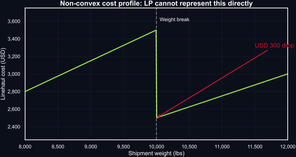

Figure 16: The linehaul cost drops at the 10,000 lb weight break, creating a non-convex profile that LP cannot represent directly.

The drop at 10,000 lbs makes this function non-convex. A standard LP requires the feasible region and objective to be convex. We need a technique that encodes this cost structure inside an LP/MIP framework.

That technique is piecewise linear approximation (Williams 2013).

The Core Idea: Approximate With Line Segments

Any nonlinear single-variable function can be approximated by connecting a series of breakpoints with straight lines.

apply_chart_style()

x_smooth = np.linspace(0, 2.5, 300)
y_smooth = x_smooth ** 2
x_focus = 1.5

breakpoint_grids = [
    np.array([0.0, 1.25, 2.5]),
    np.array([0.0, 1.0, 2.0, 2.5]),
    np.array([0.0, 0.5, 1.0, 1.5, 2.0, 2.5]),
    np.arange(0.0, 2.51, 0.25),
]
panel_titles = [
    "Very coarse: 2 segments",
    "Coarse grid: 3 segments",
    "Medium grid: 5 segments",
    "Fine grid: 10 segments",
]

fig, axes = plt.subplots(2, 2, figsize=(12, 6.5), sharey=True, sharex=True)
axes = axes.flatten()

for ax, grid_x, panel_title in zip(axes, breakpoint_grids, panel_titles):
    grid_y = grid_x ** 2
    y_focus = np.interp(x_focus, grid_x, grid_y)
    approx_error = y_focus - x_focus ** 2

    ax.plot(x_smooth, y_smooth, color=colors["secondary"], linewidth=2.2)
    ax.plot(
        grid_x, grid_y, "o-",
        color=colors["accent"], linewidth=2.0, markersize=5, zorder=3,
    )
    ax.axvline(x_focus, color=colors["text"], linestyle="--", alpha=0.35)
    ax.plot(x_focus, y_focus, "o", color=colors["primary"], markersize=7, zorder=4)
    ax.set_title(panel_title, fontsize=14, fontweight="bold")
    ax.set_xlabel("$x$")
    ax.grid(True, alpha=0.2)
    ax.text(
        0.03, 0.93,
        f"x=1.5 → {y_focus:.3f}\nError: {approx_error:.3f}",
        transform=ax.transAxes, fontsize=11, va="top",
        color=colors["annotation"],
        path_effects=[pe.withStroke(linewidth=2, foreground=colors["text"])],
    )

for idx in (0, 2):
    axes[idx].set_ylabel("$f(x)$")

legend_handles = [
    Line2D([0], [0], color=colors["secondary"], lw=2.2, label="True curve $x^2$"),
    Line2D([0], [0], color=colors["accent"], lw=2.0, marker="o", markersize=6,
           label="Piecewise fit"),
    Line2D([0], [0], color=colors["primary"], marker="o", linestyle="None",
           markersize=7, label="Interpolated value at x=1.5"),
]
fig.legend(
    handles=legend_handles, loc="lower center", ncol=3,
    bbox_to_anchor=(0.5, 0.01), frameon=False,
)
fig.suptitle(
    "More breakpoints improve local approximation accuracy",
    fontsize=19, fontweight="bold", y=0.98,
)
plt.tight_layout(rect=[0, 0.08, 1, 0.94])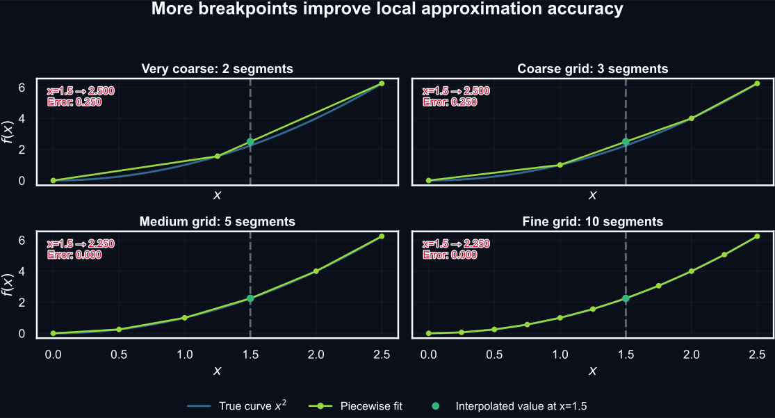

Figure 17: Piecewise approximations with 2, 3, 5, and 10 segments evaluated at x=1.5. Refinement reduces interpolation error.

Key tradeoff (Figure 17): more segments reduce error, but each breakpoint adds variables and constraints to the model.

Separable Functions

A separable function can be written as \(f(x_1, \ldots, x_n) = f_1(x_1) + \cdots + f_n(x_n)\). Each single-variable term can be independently approximated by piecewise linear segments. This is the scope of the technique.

The Lambda-Form Formulation

Given breakpoints \(a_1, a_2, \ldots, a_{K}\) with function values \(f(a_1), \ldots, f(a_K)\), we express any point on the piecewise curve as a weighted combination of breakpoints.

Decision variables:

• \(\lambda_k \geq 0\) for \(k = 1, \ldots, K\) (weights)

Core equations:

\[ x = \sum_{k=1}^{K} a_k \, \lambda_k \tag{8}\]

\[ f(x) = \sum_{k=1}^{K} f(a_k) \, \lambda_k \tag{9}\]

\[ \sum_{k=1}^{K} \lambda_k = 1, \quad \lambda_k \geq 0 \tag{10}\]

Interpretation:

The \(\lambda_k\) values represent the “weight” assigned to each breakpoint. When exactly two adjacent \(\lambda\) values are nonzero, the solution point \((x, f(x))\) lies on the line segment connecting those two breakpoints — a convex combination of neighbors.

Equations Equation 8 and Equation 9 map the weights to one point on the piecewise curve. Equation Equation 10 ensures the weights form a proper convex combination.

Numeric Walkthrough: From Plot to Weights

Use the coarse panel in Figure 17 with breakpoints \(a = (0, 1, 2, 2.5)\) and target \(x = 1.5\).

Table 16: Lambda weights for the point at \(x = 1.5\).

\(k\)	\(a_k\)	\(f(a_k)\)	\(\lambda_k\)
1	0.0	0.00	0.00
2	1.0	1.00	0.50
3	2.0	4.00	0.50
4	2.5	6.25	0.00

\[ x = 0(0) + 1(0.5) + 2(0.5) + 2.5(0) = 1.5 \]

\[ f(x) = 0(0) + 1(0.5) + 4(0.5) + 6.25(0) = 2.5 \]

True value: \(1.5^2 = 2.25\). Approximation error: \(0.25\).

Listing 5: : Python helper that computes adjacent lambda weights for interpolation.

def lambda_between_points(
    x: float, left_x: float, right_x: float
) -> tuple[float, float]:
    span = right_x - left_x
    lam_right = (x - left_x) / span
    lam_left = 1.0 - lam_right
    return lam_left, lam_right


def test_lambda_between_points() -> None:
    lam_2, lam_3 = lambda_between_points(
        1.5, 1.0, 2.0
    )
    assert abs(lam_2 - 0.5) < 1e-9
    assert abs(lam_3 - 0.5) < 1e-9

The listing in Listing 5 computes the same weights reported in Table 16.

The Adjacency Problem

The lambda form works only if at most two adjacent \(\lambda\) values are nonzero. But nothing in Equation 8 through Equation 10 enforces this.

Why does it sometimes work anyway? For a convex function being minimized, the chord connecting non-adjacent breakpoints lies above the piecewise path through intermediate breakpoints. Any non-adjacent mixture therefore produces a worse objective than the adjacent alternative, so the optimizer avoids it by optimality alone. The same logic applies (in reverse) to concave maximization.

But this reasoning breaks down for non-convex functions — exactly the kind of cost structure that motivated this lecture.

Counterexample: Non-Convex Breakpoints

Consider the breakpoints in Table 17:

Table 17: Non-convex breakpoints where adjacency matters.

\(k\)	\(a_k\)	\(f(a_k)\)
1	0	0.0
2	1	4.0
3	2	1.0
4	3	5.0

Minimize \(f(x) = \sum_k f(a_k)\lambda_k\) subject to \(x = \sum_k a_k\lambda_k = 1.5\) and \(\sum_k \lambda_k = 1\).

Without adjacency: \(\lambda_1=0.25\), \(\lambda_3=0.75\) gives \(x=1.5\), \(f=0.75\). This point lies below the piecewise line — geometrically invalid.

With adjacency: Only \(\lambda_2=0.5\), \(\lambda_3=0.5\) is feasible at \(x=1.5\), giving \(f=2.5\). This is the correct interpolation.

The relaxed solution looks better (\(0.75 < 2.5\)) but represents a point that does not exist on the piecewise approximation.

Counterexample Visualized

apply_chart_style()

x_break = np.array([0.0, 1.0, 2.0, 3.0])
y_break = np.array([0.0, 4.0, 1.0, 5.0])
x_target = 1.5

lam_relaxed = np.array([0.25, 0.0, 0.75, 0.0])
x_relaxed = float(np.dot(x_break, lam_relaxed))
y_relaxed = float(np.dot(y_break, lam_relaxed))

lam_adjacent = np.array([0.0, 0.5, 0.5, 0.0])
x_adjacent = float(np.dot(x_break, lam_adjacent))
y_adjacent = float(np.dot(y_break, lam_adjacent))

assert abs(x_relaxed - x_target) < 1e-12
assert abs(x_adjacent - x_target) < 1e-12

fig, ax = plt.subplots(figsize=(11, 5))

ax.plot(
    x_break, y_break, "o-",
    color=colors["accent"], linewidth=2.8, markersize=8,
    label="Piecewise approximation",
)
ax.plot(
    x_relaxed, y_relaxed, "x",
    color=colors["invalid"], markersize=13, mew=2.8,
    label=f"Relaxed (no adjacency): f = {y_relaxed:.2f}", zorder=5,
)
ax.plot(
    x_adjacent, y_adjacent, "o",
    color=colors["primary"], markersize=11,
    label=f"Adjacency enforced: f = {y_adjacent:.1f}", zorder=6,
)

# Dotted line showing gap between invalid point and the polyline
y_on_line = np.interp(x_target, x_break, y_break)
ax.vlines(
    x_target, ymin=y_relaxed, ymax=y_on_line,
    colors=colors["invalid"], linestyles=":", linewidth=2, alpha=0.8,
)
ax.text(
    x_target + 0.08, (y_relaxed + y_on_line) / 2,
    f"Gap: {y_on_line - y_relaxed:.2f}", fontsize=12, color=colors["annotation"],
    path_effects=[pe.withStroke(linewidth=2, foreground=colors["text"])],
)

ax.axvline(x_target, color=colors["text"], linestyle="--", alpha=0.35)
ax.text(x_target + 0.03, 4.7, "x = 1.5", fontsize=12)

ax.set_title("Same x, different objective values by modeling choice",
             fontsize=18, fontweight="bold")
ax.set_xlabel("x")
ax.set_ylabel("f(x)")
ax.grid(True, alpha=0.3)
ax.legend(loc="lower center", bbox_to_anchor=(0.5, -0.32), ncol=3, frameon=False)
plt.tight_layout(rect=[0, 0.12, 1, 1])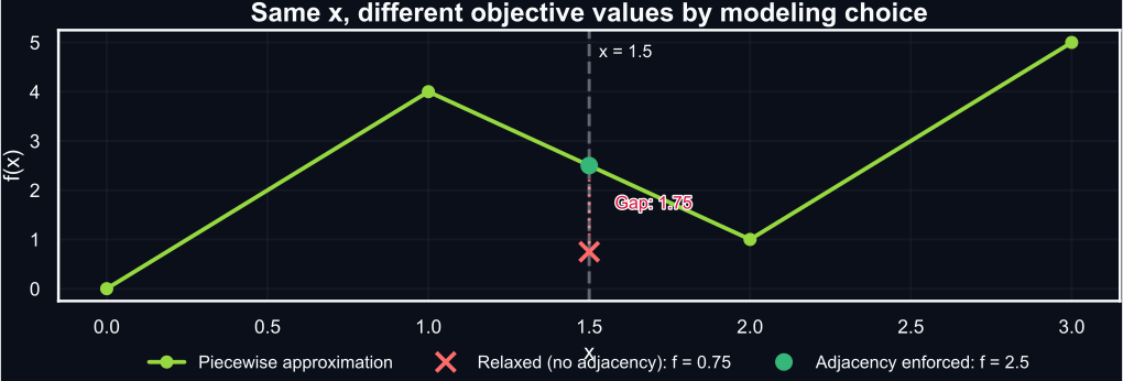

Figure 18: At x=1.5, the relaxed model (red X) picks a non-adjacent mix below the piecewise line. The adjacency-enforced model (green dot) stays on the active segment.

The dotted line in Figure 18 shows the vertical gap between the invalid non-adjacent point and the piecewise polyline.

The Adjacency Constraint: Formal Statement

Critical Requirement

At most two adjacent \(\lambda\) values can be nonzero. This keeps \((x, f(x))\) on one segment of the piecewise approximation.

Introduce binary variables \(y_r \in \{0,1\}\) for \(r = 1, \ldots, K-1\) (one per segment):

\[ \sum_{r=1}^{K-1} y_r = 1, \quad y_r \in \{0,1\} \tag{11}\]

\[ \lambda_k \leq y_{k-1} + y_k \quad \forall \, k = 1, \ldots, K \tag{12}\]

with the convention \(y_0 = y_K = 0\).

Constraint Equation 11 selects exactly one interval. Constraint Equation 12 forces each \(\lambda_k\) to zero unless it borders the active interval.

When Can You Skip Adjacency?

For convex minimization or concave maximization, the LP relaxation often respects adjacency by optimality (non-adjacent mixes produce worse objectives). For non-convex functions — like freight cost with weight breaks — adjacency must be enforced explicitly with binary variables.

Adjacency Across Function Shapes

apply_chart_style()

fig, axes = plt.subplots(1, 3, figsize=(12, 4.8))


def draw_case(
    ax: plt.Axes,
    x_break: np.ndarray,
    y_break: np.ndarray,
    x_curve: np.ndarray,
    y_curve: np.ndarray,
    title: str,
    note_text: str,
) -> None:
    ax.plot(x_curve, y_curve, color=colors["secondary"], linewidth=2.4)
    ax.plot(
        x_break, y_break, "o-",
        color=colors["accent"], linewidth=2.6, markersize=6, zorder=3,
    )

    # Adjacent interpolation: lambda_2 = lambda_3 = 0.5
    x_adj = 0.5 * x_break[1] + 0.5 * x_break[2]
    y_adj = 0.5 * y_break[1] + 0.5 * y_break[2]
    ax.plot(x_adj, y_adj, "o", color=colors["primary"], markersize=9, zorder=4)

    # Non-adjacent interpolation: lambda_1 = lambda_3 = 0.5
    x_bad = 0.5 * x_break[0] + 0.5 * x_break[2]
    y_bad = 0.5 * y_break[0] + 0.5 * y_break[2]
    y_poly = np.interp(x_bad, x_break, y_break)
    ax.plot(
        x_bad, y_bad, "x",
        color=colors["invalid"], markersize=11, mew=2.5, zorder=5,
    )
    ax.vlines(
        x_bad, ymin=min(y_bad, y_poly), ymax=max(y_bad, y_poly),
        colors=colors["invalid"], linestyles=":", linewidth=2, alpha=0.8,
    )

    ax.set_title(title, fontsize=15, fontweight="bold")
    ax.grid(True, alpha=0.25)
    ax.tick_params(axis="both", labelsize=12)
    ax.text(0.03, 0.05, note_text, transform=ax.transAxes, fontsize=11)


x_dense = np.linspace(0, 3, 200)
x_break_shape = np.array([0.0, 1.0, 2.0, 3.0])

# Convex case
convex_curve = 0.7 * x_dense ** 2 + 0.4
convex_break = 0.7 * x_break_shape ** 2 + 0.4
draw_case(
    axes[0], x_break_shape, convex_break, x_dense, convex_curve,
    "Convex minimization",
    "LP naturally returns\nadjacent lambdas.",
)
axes[0].set_ylabel("f(x)", fontsize=15, fontweight="bold")

# Concave case
concave_curve = 3.0 * np.sqrt(x_dense + 0.15)
concave_break = 3.0 * np.sqrt(x_break_shape + 0.15)
draw_case(
    axes[1], x_break_shape, concave_break, x_dense, concave_curve,
    "Concave maximization",
    "LP naturally returns\nadjacent lambdas.",
)

# Non-convex case
x_nonconv = np.array([0.0, 1.0, 2.0, 3.0])
y_nonconv = np.array([2.8, 3.5, 2.5, 3.0])
x_nonconv_dense = np.linspace(0, 3, 200)
y_nonconv_curve = np.polyval(
    np.polyfit(x_nonconv, y_nonconv, deg=3), x_nonconv_dense
)
draw_case(
    axes[2], x_nonconv, y_nonconv, x_nonconv_dense, y_nonconv_curve,
    "Non-convex / price-break",
    "Non-adjacent points can\nartificially improve objective.",
)

for ax in axes:
    ax.set_xlabel("x", fontsize=15, fontweight="bold")

legend_handles = [
    Line2D([0], [0], color=colors["secondary"], lw=2.4, label="Underlying function"),
    Line2D([0], [0], color=colors["accent"], lw=2.6, marker="o", markersize=6,
           label="Piecewise polyline"),
    Line2D([0], [0], color=colors["primary"], linestyle="None", marker="o",
           markersize=9, label="Adjacent interpolation (valid)"),
    Line2D([0], [0], color=colors["invalid"], linestyle="None", marker="x",
           markersize=11, markeredgewidth=2.5,
           label="Non-adjacent interpolation (invalid)"),
]
fig.legend(
    handles=legend_handles, loc="lower center", ncol=2,
    bbox_to_anchor=(0.5, 0.02), fontsize=12, frameon=False,
)
plt.tight_layout(rect=[0, 0.1, 1, 0.95])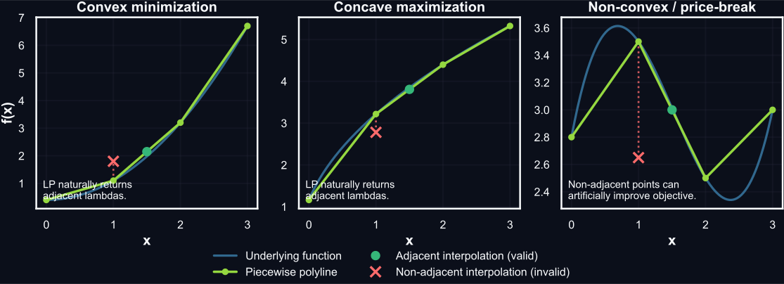

Figure 19: Three function shapes. Green dot: valid adjacent interpolation. Red X: invalid non-adjacent mix. Dotted line: vertical gap to the piecewise polyline.

Figure 19 summarizes the rule of thumb: convex-min and concave-max are often safe without explicit adjacency, but non-convex settings require the binary enforcement from Equation 11 and Equation 12.

Back to the Freight Decision: Building the Model

Now we have the tools. The freight cost function from Figure 16 is non-convex, so we need piecewise linearization with adjacency constraints.

Encoding the Discontinuity

Table 18: Breakpoints for the LTL cost model.

\(k\)	\(a_k\) (lbs)	\(f(a_k)\) (USD)
1	8,000	2,800.00
2	9,999	3,499.65
3	10,000	2,500.00
4	12,000	3,000.00
5	15,000	3,750.00

Key modeling trick: breakpoints 2 and 3 are only 1 lb apart but USD 999.65 apart. This near-vertical segment approximates the discontinuity within a formally continuous piecewise function.

• Segment 8,000–9,999: USD 35.00/CWT
• Segment 10,000+: USD 25.00/CWT

Simplification

The carrying cost term uses \(H \cdot (x - D)\), charging holding cost on the full excess for the entire period. If excess is consumed uniformly, the average excess is \((x-D)/2\) and the cost halves. We use the simpler form here; the qualitative insight is the same, but the exact break-even threshold changes.

LTL Mathematical Model

Sets and Parameters

• \(\mathcal{K} = \{1, \ldots, 5\}\): breakpoint indices; \(\mathcal{R} = \{1, \ldots, 4\}\): interval indices
• \(W_k\): weight breakpoints (lbs), from Table 18
• \(T_k\): transport cost at breakpoints (USD), from Table 18
• \(D = 8{,}000\) lbs (weekly demand), \(H = 0.11\) USD/lb/week (carrying cost), \(U = 15{,}000\) lbs (capacity)

Formulation

\[\begin{aligned} \min \quad & \sum_{k \in \mathcal{K}} T_k \lambda_k + H (x - D) && \text{(transport + carrying)} \\ \text{s.t.} \quad & x = \sum_{k \in \mathcal{K}} W_k \lambda_k && \text{(define shipment)} \\ & \sum_{k \in \mathcal{K}} \lambda_k = 1 && \text{(convex combination)} \\ & \lambda_k \leq y_{k-1} + y_k \; \forall k \in \mathcal{K} && \text{(adjacency)} \\ & \sum_{r \in \mathcal{R}} y_r = 1 && \text{(one active interval)} \\ & D \leq x \leq U && \text{(demand and capacity)} \\ & \lambda_k \geq 0,\; y_r \in \{0, 1\} && \text{(domains)} \end{aligned}\]

Quick Managerial Cross-Check

Before solving, a back-of-the-envelope calculation:

\[ H^* = \frac{\text{Freight saving}}{\text{Extra weight}} = \frac{2{,}800 - 2{,}500}{10{,}000 - 8{,}000} = 0.15 \text{ USD/lb/week} \tag{13}\]

Since \(H = 0.11 < H^* = 0.15\), the carrying cost is below the break-even threshold, so bumping to 10,000 lbs should be profitable.

Let’s verify with the optimization model.

LTL PuLP Implementation

import pulp

breakpoints = [8000, 9999, 10000, 12000, 15000]
costs = [
    breakpoints[0] / 100 * rate_below_break,
    breakpoints[1] / 100 * rate_below_break,
    breakpoints[2] / 100 * rate_at_or_above_break,
    breakpoints[3] / 100 * rate_at_or_above_break,
    breakpoints[4] / 100 * rate_at_or_above_break,
]

demand = 8000
holding_cost = 0.11
capacity = 15000
K = len(breakpoints)

prob = pulp.LpProblem("LTL_Freight_Tradeoff", pulp.LpMinimize)

lam = [pulp.LpVariable(f"lam{k}", lowBound=0) for k in range(K)]
y = [pulp.LpVariable(f"y{r}", cat="Binary") for r in range(K - 1)]
x = pulp.LpVariable("x", lowBound=0)

transport_cost = pulp.lpSum(costs[k] * lam[k] for k in range(K))
carrying_cost = holding_cost * (x - demand)
prob += transport_cost + carrying_cost, "Total_Cost"

prob += x == pulp.lpSum(breakpoints[k] * lam[k] for k in range(K))
prob += pulp.lpSum(lam) == 1

for k in range(K):
    if k == 0:
        prob += lam[k] <= y[k]
    elif k == K - 1:
        prob += lam[k] <= y[k - 1]
    else:
        prob += lam[k] <= y[k - 1] + y[k]

prob += pulp.lpSum(y) == 1
prob += x >= demand
prob += x <= capacity

prob.solve(pulp.PULP_CBC_CMD(msg=0))

LTL Solution

print(f"Status: {pulp.LpStatus[prob.status]}")
print(f"\nOptimal shipment: {x.varValue:,.0f} lbs")

transport = sum(costs[k] * lam[k].varValue for k in range(K))
holding = holding_cost * (x.varValue - demand)
total = transport + holding

print(f"Transportation cost: USD {transport:,.2f}")
print(f"Carrying cost: USD {holding:,.2f}")
print(f"Total relevant cost: USD {total:,.2f}")

freight_at_demand = demand / 100 * rate_below_break
freight_at_break = 10000 / 100 * rate_at_or_above_break
extra_weight = 10000 - demand
freight_saving = freight_at_demand - freight_at_break
h_star = freight_saving / extra_weight

print(f"\nBreak-even H*: {h_star:.4f} USD/lb/week")
print(f"Current H: {holding_cost:.4f} USD/lb/week")
decision = "Bump to 10,000 lbs" if x.varValue >= 9999.5 else "Ship demand only"
print(f"Decision: {decision}")

Status: Optimal

Optimal shipment: 10,000 lbs
Transportation cost: USD 2,500.00
Carrying cost: USD 220.00
Total relevant cost: USD 2,720.00

Break-even H*: 0.1500 USD/lb/week
Current H: 0.1100 USD/lb/week
Decision: Bump to 10,000 lbs

LTL Visualization

apply_chart_style()

weights_plot = np.linspace(8000, 15000, 400)
transport_plot = np.array([linehaul_cost(w) for w in weights_plot])
h_low = 0.10
h_high = 0.20
total_low = transport_plot + h_low * (weights_plot - demand)
total_high = transport_plot + h_high * (weights_plot - demand)

fig, ax = plt.subplots(figsize=(11, 5.5))
ax.plot(
    weights_plot, transport_plot, "--",
    color=colors["secondary"], linewidth=2.5, label="Linehaul only",
)
ax.plot(
    weights_plot, total_low,
    color=colors["primary"], linewidth=2.8,
    label="Total cost, H = 0.10 USD/lb/week",
)
ax.plot(
    weights_plot, total_high,
    color=colors["accent"], linewidth=2.8,
    label="Total cost, H = 0.20 USD/lb/week",
)

idx_low = int(np.argmin(total_low))
idx_high = int(np.argmin(total_high))
ax.plot(weights_plot[idx_low], total_low[idx_low], "o",
        color=colors["primary"], markersize=11)
ax.plot(weights_plot[idx_high], total_high[idx_high], "o",
        color=colors["accent"], markersize=11)

ax.axvline(10000, color=colors["text"], linestyle="--", alpha=0.4)
ax.text(10025, min(total_high) + 40, "10,000 lb break", fontsize=12,
        color=colors["annotation"],
        path_effects=[pe.withStroke(linewidth=2, foreground=colors["text"])])

ax.set_xlabel("Shipment weight (lbs)")
ax.set_ylabel("Cost (USD)")
ax.set_title("Freight Purchasing Tradeoff",
             fontsize=18, fontweight="bold")
ax.xaxis.set_major_formatter(StrMethodFormatter("{x:,.0f}"))
ax.yaxis.set_major_formatter(StrMethodFormatter("{x:,.0f}"))
ax.legend(loc="upper left")
ax.grid(True, alpha=0.3)
plt.tight_layout()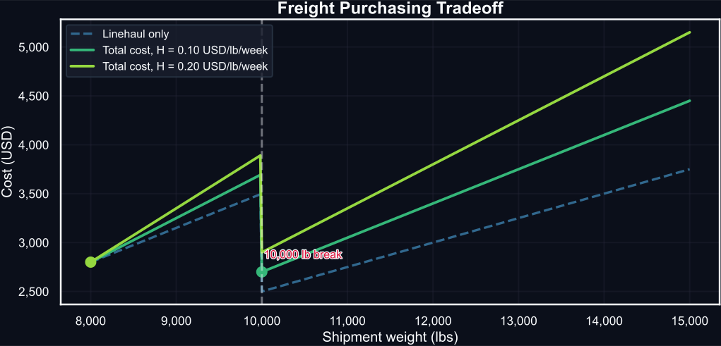

Figure 20: Linehaul cost and total cost (linehaul + carrying) under two carrying-cost assumptions. Low carrying cost supports the bump; high carrying cost does not.

Managerial Insight

With \(H = 0.11\), the model chooses 10,000 lbs. Freight saving: USD 300. Carrying cost for the extra 2,000 lbs: USD 220. Net gain: USD 80.

Figure 20 shows the sensitivity: low carrying cost supports the bump, high carrying cost keeps orders near demand. Adjacency constraints are required because the cost profile is non-convex.

Application

Taxi Rebalancing with Diminishing Returns

A Fleet Dispatching Decision

In a ride-hailing system, the marginal value of sending a vehicle to a zone decreases with the number already there: see Table 19.

Table 19: Diminishing returns per additional taxi.

Taxis sent	Marginal value (EUR)
1st	15
2nd	12
3rd	8
4th	5
5th	3
6th+	0

Why diminishing? The first taxi serves the highest-value customer. Each additional taxi competes for the remaining demand. Beyond the 5th, there is no demand left.

Given: 8 available taxis, EUR 2 per vehicle rebalancing cost.

Question: How many should we send?

This is a concave value function — the opposite shape from the freight cost problem. Both can be modeled with piecewise linearization.

Constructing Cumulative Value

Convert the marginal values from Table 19 into cumulative breakpoints (Table 20). We include breakpoint \(a_7 = 8\) matching the fleet limit so the feasible domain is fully covered.

Table 20: Breakpoints for cumulative taxi value.

\(k\)	Taxis \(a_k\)	Cumulative \(f(a_k)\) (EUR)
1	0	0
2	1	15
3	2	27
4	3	35
5	4	40
6	5	43
7	8	43

Calculation:

• \(f(1) = 15\)
• \(f(2) = 15 + 12 = 27\)
• \(f(3) = 27 + 8 = 35\)
• \(f(4) = 35 + 5 = 40\)
• \(f(5) = 40 + 3 = 43\)
• \(f(8) = 43\) (no value beyond 5)

The final breakpoint extends to 8 (the fleet size) rather than stopping at 5. This ensures the model’s feasible domain covers the entire fleet. The flat segment from 5 to 8 tells the optimizer that sending more than 5 taxis produces no additional revenue.

marginal = [15, 12, 8, 5, 3]
cumulative = [0] + [sum(marginal[:i+1]) for i in range(len(marginal))] + [43]
assert cumulative == [0, 15, 27, 35, 40, 43, 43]

Taxi Mathematical Model

Sets and Parameters

• \(\mathcal{K} = \{1, \ldots, 7\}\): breakpoint indices; \(\mathcal{R} = \{1, \ldots, 6\}\): interval indices
• \(Q_k\): taxi breakpoints, \(Q = (0, 1, 2, 3, 4, 5, 8)\)
• \(G_k\): cumulative value (EUR), \(G = (0, 15, 27, 35, 40, 43, 43)\)
• \(C^{\mathrm{reb}} = 2\) EUR/taxi; \(U = 8\) taxis

Formulation

\[\begin{aligned} \max \quad & \sum_{k \in \mathcal{K}} G_k \, \lambda_k - C^{\mathrm{reb}} \cdot x && \text{(net value)} \\ \text{s.t.} \quad & x = \sum_{k \in \mathcal{K}} Q_k \, \lambda_k && \text{(define } x \text{)} \\ & \sum_{k \in \mathcal{K}} \lambda_k = 1 && \text{(convex combination)} \\ & \lambda_k \leq y_{k-1} + y_k \; \forall k \in \mathcal{K} && \text{(adjacency)} \\ & \sum_{r \in \mathcal{R}} y_r = 1 && \text{(select interval)} \\ & x \leq U && \text{(fleet limit)} \\ & x, \lambda_k \geq 0,\; y_r \in \{0,1\} && \text{(domains)} \end{aligned}\]

Taxi PuLP Implementation

breakpoints_taxi = [0, 1, 2, 3, 4, 5, 8]
values = [0, 15, 27, 35, 40, 43, 43]
rebalancing_cost = 2
fleet_size = 8
K_taxi = len(breakpoints_taxi)

prob_taxi = pulp.LpProblem("Taxi_Rebalancing", pulp.LpMaximize)

lam_taxi = [pulp.LpVariable(f"lam{k}", lowBound=0) for k in range(K_taxi)]
y_taxi = [pulp.LpVariable(f"y{r}", cat="Binary") for r in range(K_taxi - 1)]
x_taxi = pulp.LpVariable("x", lowBound=0)

prob_taxi += (
    pulp.lpSum(values[k] * lam_taxi[k] for k in range(K_taxi))
    - rebalancing_cost * x_taxi
)

prob_taxi += x_taxi == pulp.lpSum(
    breakpoints_taxi[k] * lam_taxi[k] for k in range(K_taxi)
)
prob_taxi += pulp.lpSum(lam_taxi) == 1

for k in range(K_taxi):
    if k == 0:
        prob_taxi += lam_taxi[k] <= y_taxi[k]
    elif k == K_taxi - 1:
        prob_taxi += lam_taxi[k] <= y_taxi[k - 1]
    else:
        prob_taxi += lam_taxi[k] <= y_taxi[k - 1] + y_taxi[k]

prob_taxi += pulp.lpSum(y_taxi) == 1
prob_taxi += x_taxi <= fleet_size

prob_taxi.solve(pulp.PULP_CBC_CMD(msg=0))

Taxi Solution

print(f"Status: {pulp.LpStatus[prob_taxi.status]}")
print(f"\nOptimal decision: Send {x_taxi.varValue:.0f} taxis")

value_comp = sum(values[k] * lam_taxi[k].varValue for k in range(K_taxi))
cost_comp = rebalancing_cost * x_taxi.varValue
net = pulp.value(prob_taxi.objective)

print(f"\nExpected value: EUR {value_comp:.2f}")
print(f"Rebalancing cost: EUR {cost_comp:.2f}")
print(f"Net value: EUR {net:.2f}")

marginals = [15, 12, 8, 5, 3, 0]
x_int = int(x_taxi.varValue)
if 1 <= x_int <= 5:
    print(f"\nMarginal analysis:")
    print(f"  Value of taxi #{x_int}: EUR {marginals[x_int-1]}")
    print(f"  Cost of taxi #{x_int}: EUR {rebalancing_cost}")
    print(f"  Net benefit: EUR {marginals[x_int-1] - rebalancing_cost}")
if x_int < 6:
    next_val = marginals[x_int] if x_int < len(marginals) else 0
    print(f"  Value of taxi #{x_int+1}: EUR {next_val}")
    print(f"  Cost of taxi #{x_int+1}: EUR {rebalancing_cost}")
    print(f"  Net benefit: EUR {next_val - rebalancing_cost} → do not send")

Status: Optimal

Optimal decision: Send 5 taxis

Expected value: EUR 43.00
Rebalancing cost: EUR 10.00
Net value: EUR 33.00

Marginal analysis:
  Value of taxi #5: EUR 3
  Cost of taxi #5: EUR 2
  Net benefit: EUR 1
  Value of taxi #6: EUR 0
  Cost of taxi #6: EUR 2
  Net benefit: EUR -2 → do not send

Taxi Visualization

apply_chart_style()

fig, (ax1, ax2) = plt.subplots(1, 2, figsize=(12, 5))

# Left: Marginal value
taxis_range = list(range(0, 6))
marginal_values = [15, 12, 8, 5, 3, 0]

ax1.step(taxis_range, marginal_values, where="post", color=colors["secondary"],
         linewidth=2.5, label="Marginal value")
ax1.fill_between(taxis_range, marginal_values, step="post",
                 alpha=0.2, color=colors["secondary"])
ax1.axhline(rebalancing_cost, color=colors["accent"], linestyle="--",
            label=f"Rebalancing cost: EUR {rebalancing_cost}")

ax1.set_xlabel("Number of taxis", fontsize=15, fontweight="bold")
ax1.set_ylabel("Marginal value (EUR)", fontsize=15, fontweight="bold")
ax1.set_title("Marginal Value: Diminishing Returns",
              fontsize=18, fontweight="bold")
ax1.grid(True, alpha=0.3)
ax1.tick_params(axis="both", labelsize=13)
ax1.legend(loc="upper right", fontsize=12)

# Right: Cumulative value
ax2.plot(breakpoints_taxi, values, "o-", color=colors["primary"],
         linewidth=2.5, markersize=8, label="Cumulative value")

opt_x_taxi = x_taxi.varValue
opt_value = sum(values[k] * lam_taxi[k].varValue for k in range(K_taxi))
ax2.plot(opt_x_taxi, opt_value, "o", color=colors["accent"],
         markersize=12, label=f"Optimal: {opt_x_taxi:.0f} taxis", zorder=4)

ax2.set_xlabel("Number of taxis", fontsize=15, fontweight="bold")
ax2.set_ylabel("Cumulative value (EUR)", fontsize=15, fontweight="bold")
ax2.set_title("Cumulative Value Function", fontsize=18, fontweight="bold")
ax2.grid(True, alpha=0.3)
ax2.tick_params(axis="both", labelsize=13)
ax2.legend(loc="lower right", fontsize=12)

plt.tight_layout()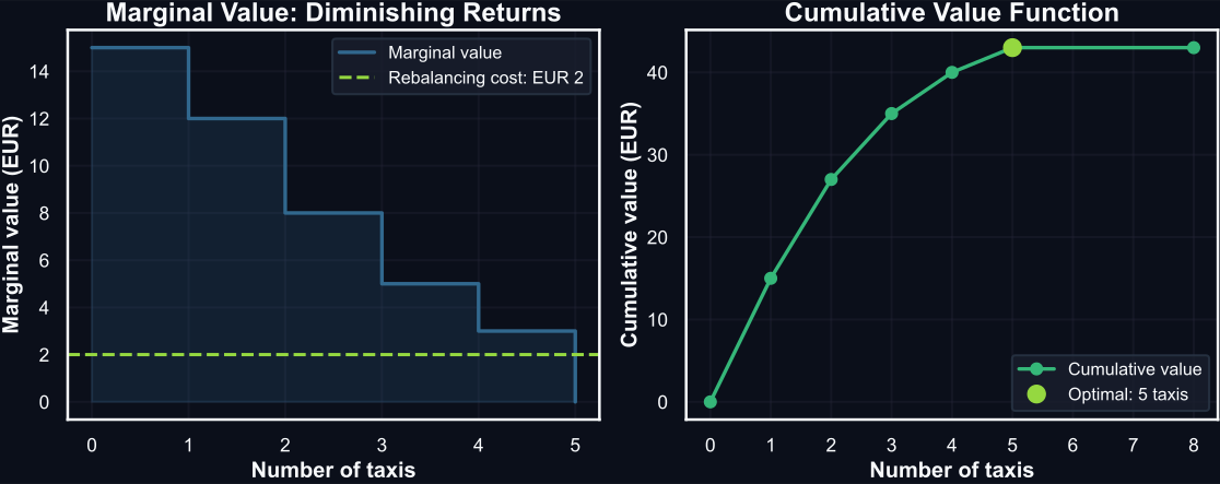

Figure 21: Left: Marginal value per taxi with the cost threshold. Right: Cumulative value with optimal dispatch point.

Economic Interpretation

Optimal decision: Send 5 taxis.

The 5th taxi: marginal value EUR 3, cost EUR 2, net EUR 1 — send it. The 6th taxi: marginal value EUR 0, cost EUR 2, net −EUR 2 — do not send.

Rule: Stop when marginal value drops below marginal cost.

Does Adjacency Matter for the Taxi Problem?

The taxi value function is concave. From the theory: concave maximization should naturally respect adjacency. Let’s verify by solving the same model without adjacency constraints and comparing.

# Solve without adjacency constraints
prob_no_adj = pulp.LpProblem("Taxi_No_Adjacency", pulp.LpMaximize)
lam_no = [pulp.LpVariable(f"lam_na{k}", lowBound=0) for k in range(K_taxi)]
x_no = pulp.LpVariable("x_na", lowBound=0)

prob_no_adj += (
    pulp.lpSum(values[k] * lam_no[k] for k in range(K_taxi))
    - rebalancing_cost * x_no
)
prob_no_adj += x_no == pulp.lpSum(
    breakpoints_taxi[k] * lam_no[k] for k in range(K_taxi)
)
prob_no_adj += pulp.lpSum(lam_no) == 1
prob_no_adj += x_no <= fleet_size

prob_no_adj.solve(pulp.PULP_CBC_CMD(msg=0))

print("WITH adjacency constraints:")
print(f"  x = {x_taxi.varValue:.1f}, net value = EUR {pulp.value(prob_taxi.objective):.2f}")
active_adj = [(k, lam_taxi[k].varValue) for k in range(K_taxi)
              if lam_taxi[k].varValue > 0.001]
print(f"  Active lambdas: {active_adj}")

print("\nWITHOUT adjacency constraints:")
print(f"  x = {x_no.varValue:.1f}, net value = EUR {pulp.value(prob_no_adj.objective):.2f}")
active_no = [(k, lam_no[k].varValue) for k in range(K_taxi)
             if lam_no[k].varValue > 0.001]
print(f"  Active lambdas: {active_no}")

same = abs(pulp.value(prob_taxi.objective) - pulp.value(prob_no_adj.objective)) < 0.01
print(f"\nSame solution? {same}")
if same:
    print("Concave maximization naturally respects adjacency here.")

WITH adjacency constraints:
  x = 5.0, net value = EUR 33.00
  Active lambdas: [(5, 1.0)]

WITHOUT adjacency constraints:
  x = 5.0, net value = EUR 33.00
  Active lambdas: [(5, 1.0)]

Same solution? True
Concave maximization naturally respects adjacency here.

Application

Parcel Band Pricing: When Bumping Cannot Help

Example 3: Nondecreasing Band Pricing

Not every tiered pricing structure creates a bump incentive. Consider the published FedEx Netherlands domestic parcel rates (“other packaging material”) (FedEx 2026), where the per-kg rate is flat within each band and nondecreasing across bands.

The data below is parsed from the published rate card.

fig, (ax1, ax2) = plt.subplots(1, 2, figsize=(12, 5))

# Left panel: rate per kg (step function)
for rates, label, color in [
    (fedex_first_rate, "FedEx First", colors["secondary"]),
    (priority_express_rate, "Priority Express", colors["primary"]),
    (priority_rate, "Priority", colors["accent"]),
]:
    ax1.step(weights_kg, rates, where="post", color=color,
             linewidth=2.4, label=label)

ax1.set_title("Published EUR/kg rate by band",
              fontsize=16, fontweight="bold")
ax1.set_xlabel("Shipment weight (kg)", fontsize=14)
ax1.set_ylabel("Rate (EUR/kg)", fontsize=14)
ax1.grid(True, alpha=0.3)
ax1.tick_params(axis="both", labelsize=12)
ax1.legend(fontsize=10, loc="lower right")

# Right panel: total charge
for total, label, color in [
    (first_total, "FedEx First", colors["secondary"]),
    (express_total, "Priority Express", colors["primary"]),
    (priority_total, "Priority", colors["accent"]),
]:
    ax2.plot(weights_kg, total, color=color, linewidth=2.6, label=label)

ax2.set_title("Implied total charge (rate × weight)",
              fontsize=16, fontweight="bold")
ax2.set_xlabel("Shipment weight (kg)", fontsize=14)
ax2.set_ylabel("Charge (EUR)", fontsize=14)
ax2.grid(True, alpha=0.3)
ax2.tick_params(axis="both", labelsize=12)
ax2.legend(fontsize=10, loc="upper left")

plt.tight_layout()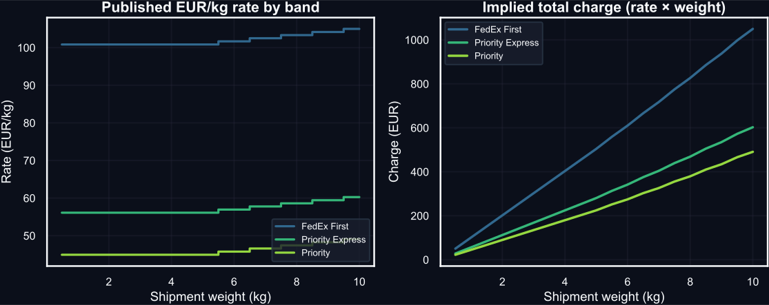

Figure 22: FedEx Netherlands domestic parcel rates. Left: per-kg rate is flat within bands and nondecreasing. Right: implied total charge is convex piecewise linear — each segment is steeper than the last.

The source document states that shipments falling between bands are charged at the higher band rate — consistent with the nondecreasing structure.

DHL Export Zones 1–3: Real-World Rate Card

The same convex pattern appears in the published DHL Express Worldwide export table for the Netherlands (DHL Express 2026). Focusing on Zones 1–3 and shipment weights from 19 kg to 70 kg gives a clean real-world piecewise linear example.

apply_chart_style()

fig, (ax1, ax2) = plt.subplots(1, 2, figsize=(12, 5.5))

for zone_name, zone_color in dhl_zone_colors.items():
    slopes = dhl_band_slopes[zone_name]
    slope_profile = np.append(slopes, slopes[-1])
    ax1.step(
        dhl_band_edges,
        slope_profile,
        where="post",
        color=zone_color,
        linewidth=2.5,
        label=zone_name,
    )
    ax1.fill_between(
        dhl_band_edges,
        slope_profile,
        step="post",
        alpha=0.10,
        color=zone_color,
    )

    for x_center, slope in zip(dhl_band_centers, slopes):
        ax1.text(
            x_center,
            slope + 0.12,
            f"{slope:.2f}",
            color=zone_color,
            fontsize=11,
            ha="center",
            path_effects=[
                pe.withStroke(linewidth=2, foreground=colors["background"])
            ],
        )

for band_break in [20.0, 30.0]:
    ax1.axvline(band_break, color=colors["text"], linestyle="--", alpha=0.3)
    ax2.axvline(band_break, color=colors["text"], linestyle="--", alpha=0.3)

ax1.set_title("Implied slope by tariff band", fontsize=16, fontweight="bold")
ax1.set_xlabel("Shipment weight (kg)", fontsize=14)
ax1.set_ylabel("Marginal charge (EUR/kg)", fontsize=14)
ax1.set_xlim(19.0, 70.0)
ax1.grid(True, alpha=0.3)
ax1.tick_params(axis="both", labelsize=12)
ax1.legend(fontsize=11, loc="upper left")

for zone_name, charges in dhl_zone_charges.items():
    zone_color = dhl_zone_colors[zone_name]
    ax2.plot(
        dhl_dense_weights,
        dhl_dense_charges[zone_name],
        color=zone_color,
        linewidth=2.6,
    )
    ax2.plot(
        dhl_weights_kg,
        charges,
        "o",
        color=zone_color,
        markersize=5.5,
        label=zone_name,
    )

ax2.set_title("Published total export charge", fontsize=16, fontweight="bold")
ax2.set_xlabel("Shipment weight (kg)", fontsize=14)
ax2.set_ylabel("Charge (EUR)", fontsize=14)
ax2.set_xlim(19.0, 70.0)
ax2.grid(True, alpha=0.3)
ax2.tick_params(axis="both", labelsize=12)
ax2.legend(fontsize=11, loc="upper left")
ax2.xaxis.set_major_formatter(StrMethodFormatter("{x:,.0f}"))
ax2.yaxis.set_major_formatter(StrMethodFormatter("{x:,.0f}"))

plt.tight_layout()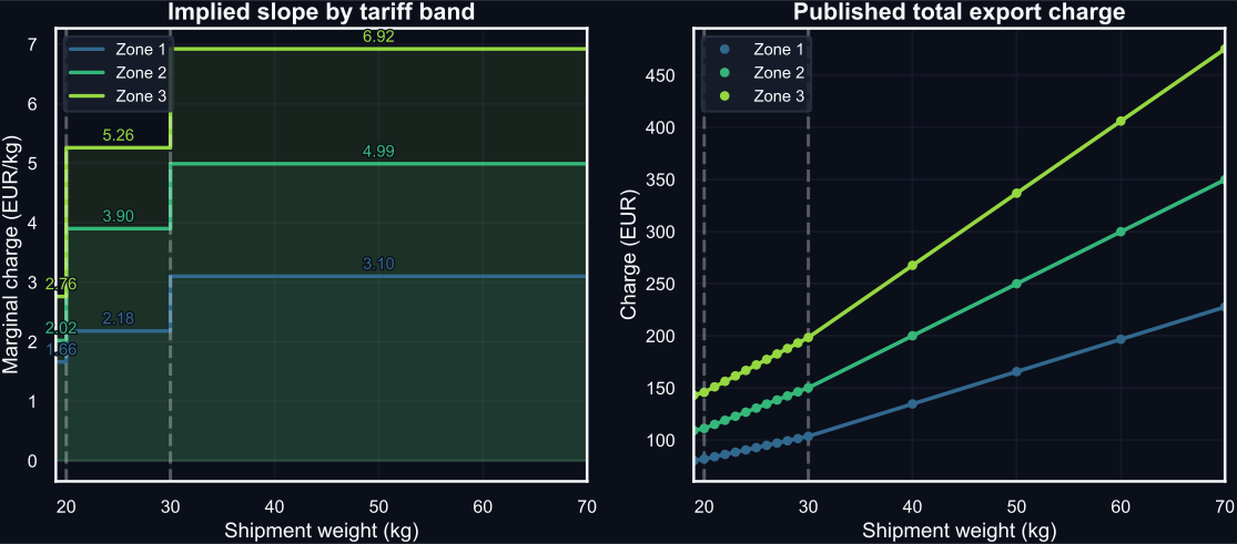

Figure 23: DHL Express Worldwide export rates for the Netherlands, Zones 1–3. Left: slope of the tariff, expressed as EUR/kg equivalent, rises at 20 kg and 30 kg. Right: total charge is piecewise linear and convex over the published range.

The breakpoints at 20 kg and 30 kg increase the marginal charge in every zone, so the DHL tariff over this range is a convex piecewise linear cost function. That makes it a useful real-world contrast with the LTL “all-units discount” case, where the cost curve drops instead of steepening.

Why There Is No Bump Incentive

The critical difference from the LTL example is the shape of the total cost function.

In the OR literature, pricing schedules fall into two canonical types (Munson and Rosenblatt 1998; Croxton et al. 2003):

All-units discount — the lower rate applies to the entire order once a threshold is crossed. Total cost drops at the break. This is the LTL freight case: the cost function is non-convex, and over-ordering (“bumping”) to capture the lower rate can be rational.

Incremental / nondecreasing band pricing — each band’s rate applies only within that band, and rates do not decrease. Total cost never drops. This is the FedEx NL parcel case: the cost function is convex piecewise linear.

fig, (ax1, ax2) = plt.subplots(1, 2, figsize=(12, 5))

# Left: all-units discount (LTL style)
q_all = np.linspace(0, 150, 500)
cost_all = np.where(q_all < 100, 10 * q_all, 8 * q_all)

ax1.plot(q_all, cost_all, color=colors["accent"], linewidth=2.8)
ax1.axvline(100, color=colors["text"], linestyle="--", alpha=0.4)
ax1.annotate(
    "Cost drops\nat break",
    xy=(100, 800), xytext=(60, 600),
    fontsize=13, color=colors["invalid"],
    arrowprops=dict(arrowstyle="->", color=colors["invalid"], lw=2),
)
ax1.set_title("All-units discount (LTL freight)",
              fontsize=16, fontweight="bold")
ax1.set_xlabel("Quantity", fontsize=14)
ax1.set_ylabel("Total cost", fontsize=14)
ax1.grid(True, alpha=0.3)
ax1.tick_params(axis="both", labelsize=12)
ax1.text(
    0.03, 0.92, "Non-convex\nBump incentive exists",
    transform=ax1.transAxes, fontsize=12, color=colors["invalid"],
    va="top", fontweight="bold",
)

# Right: nondecreasing band pricing (parcel style)
q_inc = np.linspace(0, 150, 500)
cost_inc = np.where(q_inc <= 100, 8 * q_inc, 800 + 10 * (q_inc - 100))

ax2.plot(q_inc, cost_inc, color=colors["primary"], linewidth=2.8)
ax2.axvline(100, color=colors["text"], linestyle="--", alpha=0.4)
ax2.set_title("Nondecreasing band pricing (parcel)",
              fontsize=16, fontweight="bold")
ax2.set_xlabel("Quantity", fontsize=14)
ax2.set_ylabel("Total cost", fontsize=14)
ax2.grid(True, alpha=0.3)
ax2.tick_params(axis="both", labelsize=12)
ax2.text(
    0.03, 0.92, "Convex\nNo bump incentive",
    transform=ax2.transAxes, fontsize=12, color=colors["primary"],
    va="top", fontweight="bold",
)

plt.tight_layout()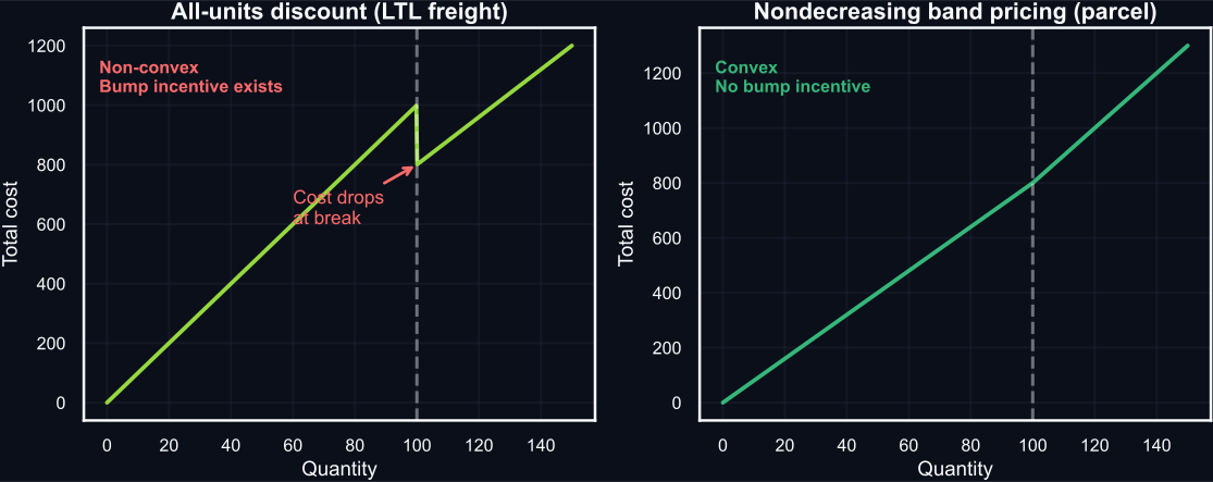

Figure 24: All-units discount (left) creates a non-convex cost drop at the break. Nondecreasing band pricing (right) produces a convex cost curve with no drop.

Under nondecreasing band pricing, every additional unit costs at least as much as the previous one. Over-declaring weight only increases the charge. There is no weight threshold where the total cost drops, so there is nothing to “game.”

Modeling Consequence

When the cost function is convex and you are minimizing, the LP relaxation already respects adjacency. No binary variables are needed — the problem reduces to a standard LP. This makes convex piecewise linear costs computationally much cheaper than the non-convex LTL case.

Contrasting All Three Examples

Each example produces a different function shape, and the shape determines the modeling complexity:

Table 21: Three function shapes and their modeling implications.

	LTL Freight	Taxi Rebalancing	Parcel Band Pricing
Direction	Minimize cost	Maximize value	Minimize cost
Shape	Non-convex (price drop)	Concave (diminishing returns)	Convex (nondecreasing rates)
Bump/gaming?	Yes — rational to over-order	N/A	No — over-ordering always hurts
Adjacency needed?	Essential	Redundant (concave max)	Redundant (convex min)
Solver class	MIP (binary \(y_r\))	LP sufficient	LP sufficient

Practical Advice

When in doubt, include adjacency constraints. They add binary variables and make the problem a MIP, but they guarantee correctness regardless of function shape. Only omit them when you can prove the function is convex (for minimization) or concave (for maximization) over the relevant domain.

Common Pitfalls

Pitfalls to Avoid

1. Omitting adjacency for non-convex functions. The optimizer will exploit non-adjacent lambda combinations that produce artificially good objective values. The solution looks optimal but represents a point not on the piecewise curve.

2. Ignoring additive cost components. If the model includes only linehaul breakpoints but omits fixed surcharges (flat fees, accessorials), savings from a weight-break move can be overstated.

3. Too few breakpoints near the optimum. A coarse grid can produce large approximation errors. Practical strategy: solve once, refine the grid near the optimal \(x\), then re-optimize.

4. Breakpoints beyond the feasible region. Not harmful — constraints handle it — but extra breakpoints add unnecessary variables. Match the breakpoint domain to the feasible range implied by model constraints.

5. Product terms. Piecewise linearization handles \(f(x_i)\) terms. For products \(x_1 \cdot x_2\), a different transformation is needed: \(u_1 = \frac{1}{2}(x_1+x_2)\), \(u_2 = \frac{1}{2}(x_1-x_2)\), so \(x_1 x_2 = u_1^2 - u_2^2\) — then each squared term is separable.

When to Use Piecewise Linear Functions

Application Guidelines

Good fit:

• Nonlinear relationship in a single variable (separable)
• Function approximable by a modest number of linear segments (4–10)
• You want to stay within LP/MIP frameworks and avoid NLP solvers
• Volume discounts, tiered pricing, diminishing returns, progressive costs

Poor fit:

• Smooth, well-behaved function where NLP solvers work well
• Product terms \(x_1 \times x_2\) (requires a different linearization)
• Very high-dimensional nonlinearity (too many breakpoints)

Key Takeaways

Modeling technique:

• Piecewise linear approximation extends LP/MIP to handle nonlinearity
• The lambda form interpolates between breakpoints using convex weights
• Adjacency constraints (binary variables) keep the solution on the piecewise curve
• Essential for non-convex functions; often redundant for convex-min or concave-max

Applications seen:

• Freight purchasing (non-convex): weight break creates cost drop, bumping can be rational, adjacency essential
• Fleet dispatching (concave): diminishing returns, stop when marginal value falls below marginal cost, adjacency redundant
• Parcel band pricing (convex): nondecreasing rates eliminate gaming, LP sufficient, adjacency redundant
• Same lambda-form structure, same constraint pattern, but the function shape dictates complexity

Always Verify

Check approximation accuracy before using results for business decisions. Refine the grid where it matters most.

References

Ahuja, Ravindra K., Thomas L. Magnanti, and James B. Orlin. 1993. Network Flows: Theory, Algorithms, and Applications. Prentice Hall.

Arora, Jasbir S. 2017. “Multi-Objective Optimum Design Concepts and Methods.” In Introduction to Optimum Design, 4th ed. Elsevier. https://doi.org/10.1016/B978-0-12-800806-5.00018-4.

Boeing, Geoff. 2017. “OSMnx: New Methods for Acquiring, Constructing, Analyzing, and Visualizing Complex Street Networks.” Computers, Environment and Urban Systems 65: 126–39. https://doi.org/10.1016/j.compenvurbsys.2017.05.004.

Brown, Gerald G., and Robert F. Dell. 2007. “Formulating Integer Linear Programs: A Rogues’ Gallery.” INFORMS Transactions on Education 7 (2): 153–59.

Caramia, Massimiliano, and Paolo Dell’Olmo. 2008. Multi-Objective Management in Freight Logistics. Springer.

Chang, Kuang-Hua. 2015. “Multiobjective Optimization and Advanced Topics.” In Design Theory and Methods Using CAD/CAE. Elsevier. https://doi.org/10.1016/B978-0-12-398512-5.00005-0.

Chankong, Vira, and Yacov Y. Haimes. 1983. Multiobjective Decision Making: Theory and Methodology. Elsevier.

Clarke, G., and J. W. Wright. 1964. “Scheduling of Vehicles from a Central Depot to a Number of Delivery Points.” Operations Research 12 (4): 568–81.

Croxton, Keely L., Bernard Gendron, and Thomas L. Magnanti. 2003. “A Comparison of Mixed-Integer Programming Models for Nonconvex Piecewise Linear Cost Minimization Problems.” Management Science 49 (9): 1268–73. https://doi.org/10.1287/mnsc.49.9.1268.16570.

Dantzig, George B., and John H. Ramser. 1959a. “The Truck Dispatching Problem.” Management Science 6 (1): 80–91.

Dantzig, George B., and John H. Ramser. 1959b. “The Truck Dispatching Problem.” Management Science 6 (1): 80–91.

DHL Express. 2026. Service & Rate Guide 2026: Netherlands. PDF. https://www.dhlexpress.nl/sites/default/files/content/Netherlands%20English%20SARG26%20Full%20DEF.pdf.

Dijkstra, Edsger W. 1959. “A Note on Two Problems in Connexion with Graphs.” Numerische Mathematik 1: 269–71.

FedEx. 2026. Information on Your Rates and Shipments: Applicable in the Netherlands from 5 January 2026. PDF. https://www.fedex.com/content/dam/fedex/international/rates/new-offer-rates-domestic-en-nl.pdf.

Gendreau, Michel, Alain Hertz, and Gilbert Laporte. 1994. “A Tabu Search Heuristic for the Vehicle Routing Problem.” Management Science 40 (10): 1276–90.

Geoffrion, Arthur M. 1968. “Proper Efficiency and the Theory of Vector Maximization.” Journal of Mathematical Analysis and Applications 22 (3): 618–30.

Golden, Bruce L., Arjang A. Assad, Leon Levy, and Frederic G. Gheysens. 1984. “The Fleet Size and Mix Vehicle Routing Problem.” Computers & Operations Research 11 (1): 49–66.

Hitchcock, Frank L. 1941. “The Distribution of a Product from Several Sources to Numerous Localities.” Journal of Mathematics and Physics 20 (1-4): 224–30.

Lalla-Ruiz, Eduardo, and Stefan Voß. 2020. “A POPMUSIC Approach for the Multi-Depot Cumulative Capacitated Vehicle Routing Problem.” Optimization Letters 14 (3): 671–91.

Maffioli, Federico, and Anna Sciomachen. 2015. Chapter 2: Multi-Objective Optimization. PDF.

Miettinen, Kaisa. 1994. On the Methodology of Multiobjective Optimization with Applications. University of Jyväskylä.

Miller, Clair E., Albert W. Tucker, and Richard A. Zemlin. 1960. “Integer Programming Formulation of Traveling Salesman Problems.” Journal of the ACM 7 (4): 326–29.

Montoya-Torres, Jairo R., Julián López Franco, Santiago Nieto Isaza, Heriberto Felizzola Jiménez, and Nilson Herazo-Padilla. 2015. “A Literature Review on the Vehicle Routing Problem with Multiple Depots.” Computers & Industrial Engineering 79: 115–29.

Munson, Charles L., and Meir J. Rosenblatt. 1998. “Theories and Realities of Quantity Discounts: An Exploratory Study.” Production and Operations Management 7 (4): 352–69. https://doi.org/10.1111/j.1937-5956.1998.tb00127.x.

Murray, Chase C., and Amanda G. Chu. 2015. “The Flying Sidekick Traveling Salesman Problem: Optimization of Drone-Assisted Parcel Delivery.” Transportation Research Part C: Emerging Technologies 54: 86–109.

National Motor Freight Traffic Association. 2026. Freight Classification Development Council Procedures 2026. PDF. https://nmfta.org/wp-content/media/2026/01/FCDC-Procedures-2026.pdf.

OpenStreetMap Foundation. 2026. “OpenStreetMap Copyright and License.” https://www.openstreetmap.org/copyright.

Psaraftis, Harilaos N. 1980. “A Dynamic Programming Solution to the Single Vehicle Many-to-Many Immediate Request Dial-a-Ride Problem.” Transportation Science 14 (2): 130–54.

Solomon, Marius M. 1987a. “Algorithms for the Vehicle Routing and Scheduling Problems with Time Window Constraints.” Operations Research 35 (2): 254–65.

Solomon, Marius M. 1987b. “Algorithms for the Vehicle Routing and Scheduling Problems with Time Window Constraints.” Operations Research 35 (2): 254–65.

Sudhoff, Scott. 2007. Lecture 9: Multi-Objective Optimization. PDF slides.

Williams, Paul. 2013. Model Building in Mathematical Programming. 5th ed. Wiley.

Shortest Path Algorithms

Motivation

Why calculate shortest paths?

Distance Matrix as a Core Primitive

Motivation. In logistics applications, routing is called repeatedly inside optimization loops. You need fast and consistent path costs for many origin-destination pairs.

Challenge. If each query recomputes a path from scratch, dispatch and heuristic performance degrades quickly.

Solution. Precompute a distance matrix with shortest paths, then query it instantly (lookup) inside optimization models (see Figure 25).

graph LR    
    A["Raw directed<br>road graph"] --> B["Shortest-path<br>engine"]
    B --> C["Distance matrix"]
    C --> D["Routing optimization model"]

Figure 25: Routing pipeline: shortest paths feed distance matrices for optimization models.

Problem Formulation

Given a directed graph \(G=(\mathcal{V}, \mathcal{E})\) with nonnegative costs \(C_{ij}\) on arcs \((i,j)\in\mathcal{E}\), find the minimum-cost:

• Single-pair: shortest path from source \(s\) to destination \(t\)
• Single-source: shortest paths from \(s\) to all nodes
• All-pairs: repeat single-source for every origin

Example Network

In the following slides, we will solve the shortest path problem on the toy directed road network shown in Figure 26, which has 5 nodes and 7 arcs with travel times as weights.

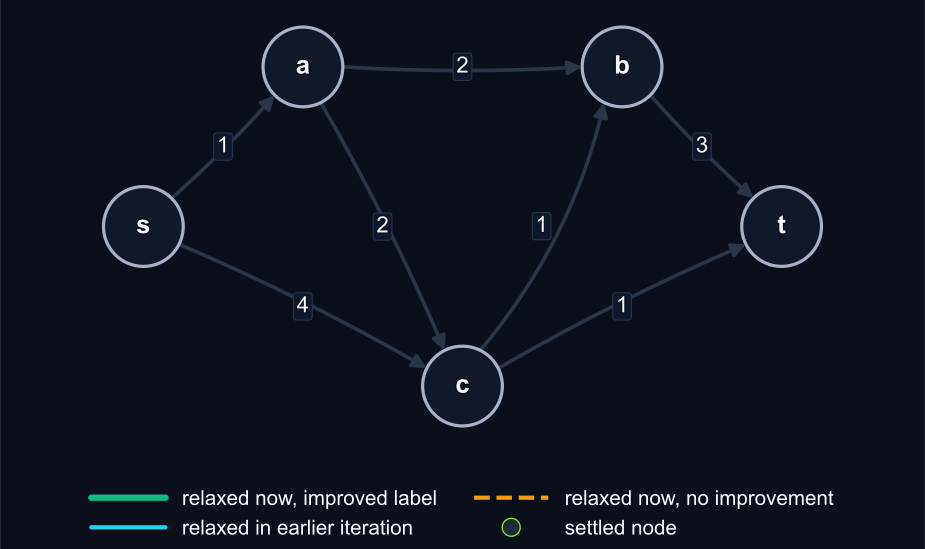
Figure 26: Directed travel network with arc weights as travel times in minutes.

The MIP Approach

Optimization

Modeling shortest paths as a 1-unit flow problem

Formulating Shortest Path as a MIP (Sets, Parameters, Variables)

We can model the shortest path problem as a special case of min-cost flow with unit demand.

Objective: send one unit of flow from \(s\) to \(t\) at minimum cost.

Sets

• \(\mathcal{V}\): nodes, indexed by \(i\)
• \(\mathcal{E}\): directed arcs, indexed by \((i,j)\)

Parameters

• \(C_{ij}\) (minutes): travel cost on arc \((i,j)\)
• \(B_i\): node balance, where \(B_s=1\), \(B_t=-1\), and \(B_i=0\) otherwise

Variables

• \(x_{ij}\): arc-use variable, binary, \(x_{ij}\in\{0,1\}\)
• \(z\) (minutes): objective value

Formulating Shortest Path as a MIP (Model)

Model

• Equation 14 defines the objective to minimize total travel time.
• Constraints in Equation 15 enforce flow balance at each node, ensuring that one unit of flow leaves the source, one unit arrives at the sink, and flow is conserved at intermediate nodes.
• The binary domain constraints in Equation 16 ensure that arcs are either used or not used in the path.

\[ \text{Minimize total cost:}\quad z = \sum_{(i,j)\in\mathcal{E}} C_{ij}x_{ij} \tag{14}\]

subject to:

\[ \sum_{j:(i,j)\in\mathcal{E}} x_{ij} - \sum_{j:(j,i)\in\mathcal{E}} x_{ji} = B_i \quad \forall i\in\mathcal{V} \quad \text{(flow balance)} \tag{15}\]

\[ x_{ij}\in\{0,1\} \quad \forall (i,j)\in\mathcal{E} \quad \text{(binary domain)} \tag{16}\]

Solving Shortest Path with MIP

Listing 6 implements the MIP formulation for the example network in Figure 26, and prints the optimal path and its cost.

Listing 6: MIP implementation of shortest path on the toy network with regression test.

import pulp as pl


def solve_shortest_path_mip() -> tuple[float, set[tuple[str, str]]]:
    # 1) Input data.
    nodes = ["s", "a", "b", "c", "t"]
    source = "s"
    sink = "t"
    costs = {
        ("s", "a"): 1,
        ("s", "c"): 4,
        ("a", "b"): 2,
        ("a", "c"): 2,
        ("c", "t"): 1,
        ("b", "t"): 3,
        ("c", "b"): 1,
    }

    # 2) Build optimization model.
    model = pl.LpProblem("shortest_path_mip", pl.LpMinimize)
    x = {}
    for arc in costs:
        var_name = f"x_{arc[0]}_{arc[1]}"
        x[arc] = pl.LpVariable(var_name, cat=pl.LpBinary)

    model += pl.lpSum(costs[arc] * x[arc] for arc in costs)

    # 3) Add flow-balance constraints.
    for node in nodes:
        out_flow = pl.lpSum(x[i, j] for (i, j) in costs if i == node)
        in_flow = pl.lpSum(x[i, j] for (i, j) in costs if j == node)
        rhs = 1 if node == source else (-1 if node == sink else 0)
        model += out_flow - in_flow == rhs

    # 4) Solve and parse the solution.
    model.solve(pl.PULP_CBC_CMD(msg=False))

    objective = float(pl.value(model.objective))
    used = {arc for arc in costs if pl.value(x[arc]) > 0.5}
    return objective, used


def test_shortest_path_mip() -> None:
    objective, used = solve_shortest_path_mip()
    assert abs(objective - 4.0) < 1e-9
    assert used == {("s", "a"), ("a", "c"), ("c", "t")}

Printed solution

Objective value: 4.0
Selected arcs:
  ('a', 'c')
  ('c', 't')
  ('s', 'a')

Why Not Just Use MIP?

• Running a MIP solver can be overkill for shortest path, which has efficient specialized algorithms.
• Performance: MIP solvers may take longer to solve large shortest path instances.

Dijkstra’s Algorithm

Graph Theory

Efficient labeling for non-negative arc costs

The Dijkstra Algorithm

• Dikstra’s algorithm is a classic method for solving shortest path problems with non-negative arc costs (Dijkstra 1959).
• It uses a label-setting approach, maintaining tentative distances and a priority queue to efficiently find the next node to settle.

Dijkstra Algorithm Flow

graph LR
    S(("Start")) --> I["Initialize<br><b>dist[source]</b>=0<br>and <b>others=inf</b>"]
    I --> H["Push source<br>into min-heap"]
    H --> Q{"Heap empty?"}
    Q -- "Yes" --> E(("Done"))
    Q -- "No" --> P["Pop node <b>u</b><br>with smallest<br><b>dist[u]</b>"]
    P --> C{"<b>u</b> already<br>settled?"}
    C -- "Yes" --> Q
    C -- "No" --> M["Mark <b>u</b><br>as settled"]
    M --> R["Relax each<br>outgoing edge<br>(<b>u</b>,<b>v</b>)"]
    R --> Q

Figure 27: Detailed Dijkstra flow from initialization to path reconstruction.

Relax¹ is the key update step in each iteration.

1. Relax edge \((u,v)\): Check whether dist[u] + cost(u,v) improves dist[v]. If yes, update dist[v] and prev[v].

Key Data Structures

For Dijkstra’s algorithm, we maintain:

• dist[v]: current best distance from source to node \(v\)
• prev[v]: predecessor pointer for path reconstruction
• Min-priority queue (heap)¹ ordered by tentative distance
• Settled² set \(\mathcal{S}\) of finalized nodes

Label-setting invariant: when a node is popped³ as current minimum, its distance is final for nonnegative arc costs (Dijkstra 1959; Ahuja et al. 1993).

This is the key correctness intuition. Repeat that nonnegative edge weights are what make the invariant valid.

1. Heap: A priority-queue data structure that returns the smallest tentative distance quickly.

2. Settled node: Node whose shortest-distance label is final.

3. Pop: Remove and read the minimum-key item from the heap.

Example Walkthrough

Considering the toy network in Figure 26, we illustrate Dijkstra’s algorithm step-by-step starting from source node s to find the shortest path to target node t.

Table 22 shows the initial state of the distance labels before any nodes are settled.

Table 22: Initialization row for Dijkstra on Figure 26. The \(\infty\) values are the starting tentative distances for all nodes except the source.

Iteration	Settled node	dist[s]	dist[a]	dist[b]	dist[c]	dist[t]
0	—	0	\(\infty\)	\(\infty\)	\(\infty\)	\(\infty\)

Figure 28: Initial graph state before settling any node.

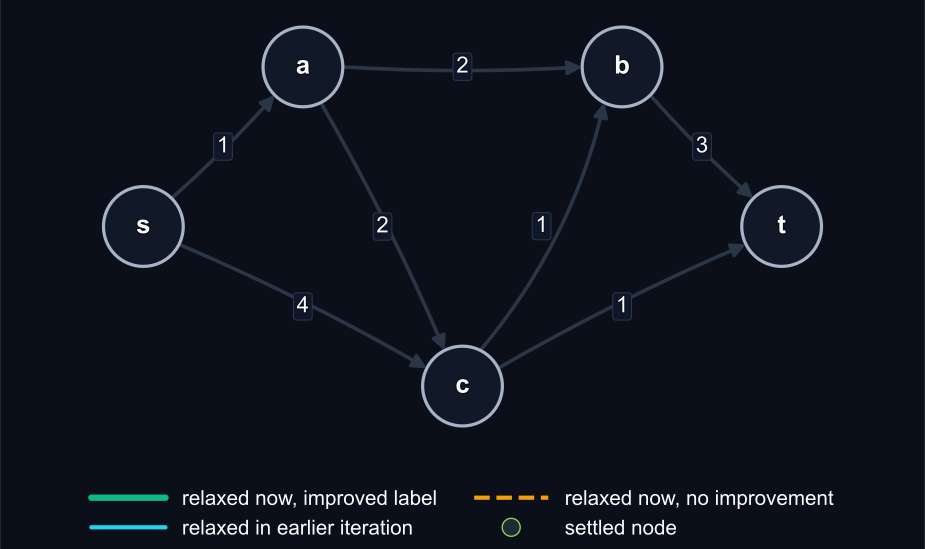
Step 1: Settle s

Relax outgoing arcs:

• \(s\to a\): dist[a]=1
• \(s\to c\): dist[c]=4

Table 23: Growing table after settling s.

Iteration	Settled node	dist[s]	dist[a]	dist[b]	dist[c]	dist[t]
0	—	0	\(\infty\)	\(\infty\)	\(\infty\)	\(\infty\)
1	s	0	1	\(\infty\)	4	\(\infty\)

Figure 29: Step 1: node s settled, edges (s,a) and (s,c) relaxed.

Iteration 1 is the first-wave relaxation from the source.

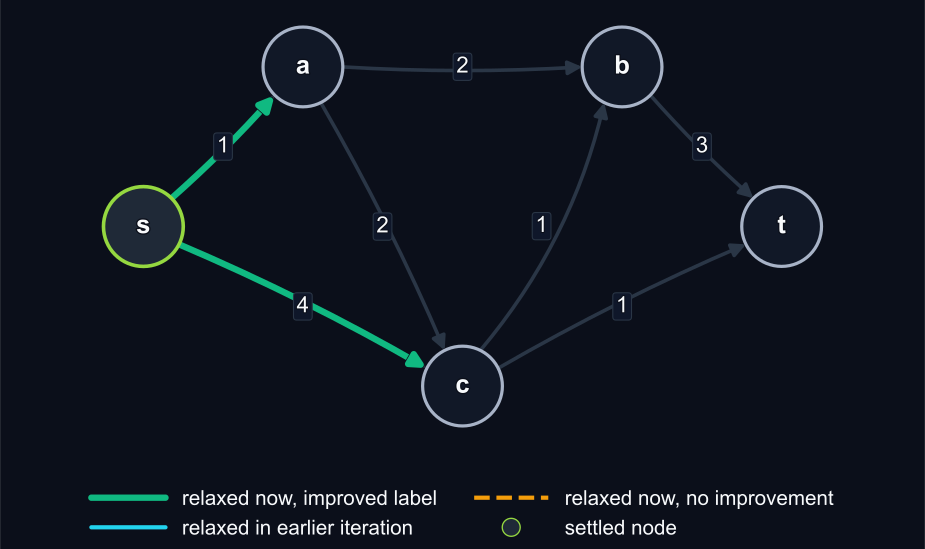
Step 2: Settle a

Relax outgoing arcs:

• \(a\to b\): dist[b]=3
• \(a\to c\): dist[c]=min(4,3)=3

Table 24: Growing table after settling a.

Iteration	Settled node	dist[s]	dist[a]	dist[b]	dist[c]	dist[t]
0	—	0	\(\infty\)	\(\infty\)	\(\infty\)	\(\infty\)
1	s	0	1	\(\infty\)	4	\(\infty\)
2	a	0	1	3	3	\(\infty\)

Figure 30: Step 2: node a settled, edges (a,b) and (a,c) relaxed.

Node c improves from 4 to 3. This is the core effect of relaxation.

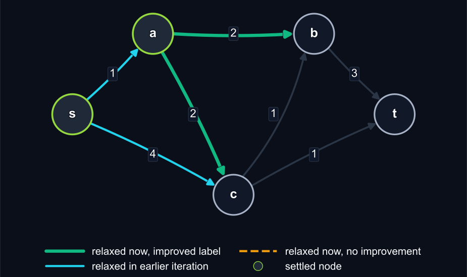
Step 3: Settle b (Tie Case)

Nodes b and c tie at 3. Suppose b is popped first.

Relax outgoing arc:

• \(b\to t\): dist[t]=6

Table 25: Growing table after settling b.

Iteration	Settled node	dist[s]	dist[a]	dist[b]	dist[c]	dist[t]
0	—	0	\(\infty\)	\(\infty\)	\(\infty\)	\(\infty\)
1	s	0	1	\(\infty\)	4	\(\infty\)
2	a	0	1	3	3	\(\infty\)
3	b	0	1	3	3	6

Figure 31: Step 3: node b settled and edge (b,t) relaxed.

First time reaching t is not final. Finality only occurs when t is popped as the minimum tentative node.

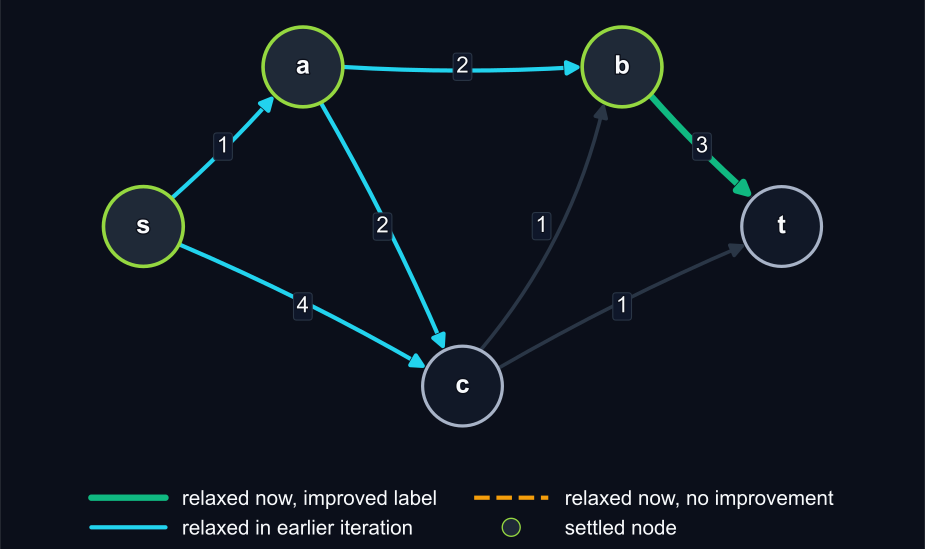
Step 4: Settle c and Improve t

Relax outgoing arcs:

• \(c\to t\): dist[t]=min(6,4)=4 improves
• \(c\to b\): candidate 4, no improvement (orange dashed edge in the figure)

Table 26: Growing table after settling c.

Iteration	Settled node	dist[s]	dist[a]	dist[b]	dist[c]	dist[t]
0	—	0	\(\infty\)	\(\infty\)	\(\infty\)	\(\infty\)
1	s	0	1	\(\infty\)	4	\(\infty\)
2	a	0	1	3	3	\(\infty\)
3	b	0	1	3	3	6
4	c	0	1	3	3	4

Figure 32: Step 4: node c settled; relaxing edge (c,t) improves t, while relaxing edge (c,b) yields no improvement.

This is the decisive iteration. The destination label drops from 6 to 4.

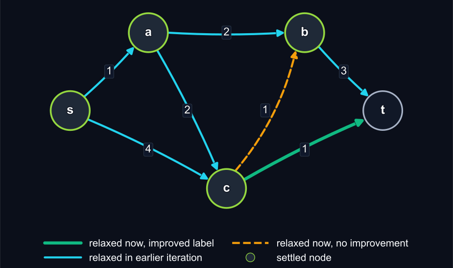
Step 5: Settle t and Reconstruct Path

Node t is now popped with label 4, so the shortest path is final.

\[ t \leftarrow c \leftarrow a \leftarrow s \]

\[ s \to a \to c \to t,\quad \text{cost } 4 \]

Table 27: Final growing table after settling t.

Iteration	Settled node	dist[s]	dist[a]	dist[b]	dist[c]	dist[t]
0	—	0	\(\infty\)	\(\infty\)	\(\infty\)	\(\infty\)
1	s	0	1	\(\infty\)	4	\(\infty\)
2	a	0	1	3	3	\(\infty\)
3	b	0	1	3	3	6
4	c	0	1	3	3	4
5	t	0	1	3	3	4

Figure 33: Final state with shortest-path edges highlighted.

The shortest path is s -> a -> c -> t. This step closes the growing-table walk-through.

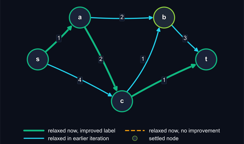
Example Walkthrough Summary

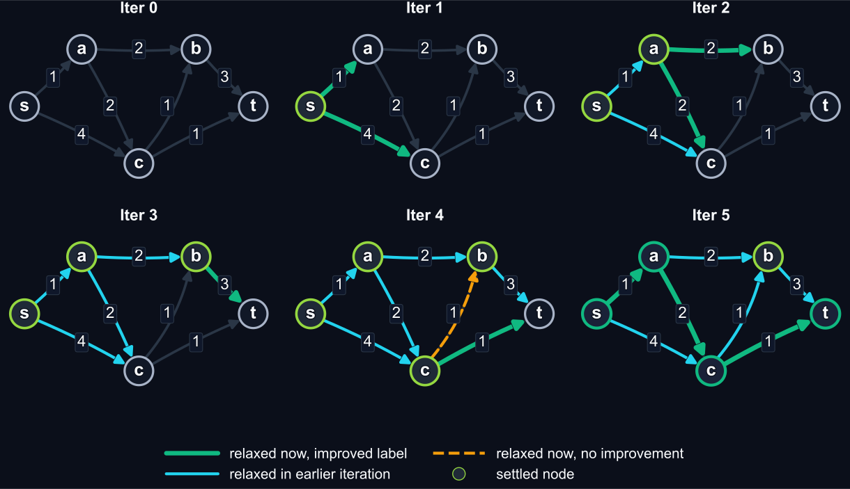
Figure 34: Complete Dijkstra trace in one panel (iterations 0–5), using settled and relaxed states.

This panel summarizes the complete label-setting progression using standard terminology: settled nodes and relaxation outcomes (Dijkstra 1959; Ahuja et al. 1993).

Implementing Dijkstra

Listing 7 shows a Python implementation of Dijkstra’s algorithm that prints the settle and relax decisions at each step, along with the evolving set of settled nodes. Listing 8 then runs the algorithm and prints the final objective value and path.

Note: Many library implementations of Dijkstra exist (e.g., in NetworkX, Boost Graph Library, etc.).

Listing 7: Heap-based Dijkstra implementation that prints settle and relax decisions.

import heapq
import math

graph = {
    "s": [("a", 1), ("c", 4)],
    "a": [("b", 2), ("c", 2)],
    "b": [("t", 3)],
    "c": [("t", 1), ("b", 1)],
    "t": [],
}


def dijkstra_with_trace(
    source: str, sink: str
) -> tuple[dict[str, float], dict[str, str | None]]:
    dist = {node: math.inf for node in graph}
    prev = {node: None for node in graph}
    dist[source] = 0.0
    heap = [(0.0, source)]
    settled = set()
    step = 0

    while heap:
        cur_dist, node = heapq.heappop(heap)
        if node in settled:
            continue
        settled.add(node)
        step += 1
        print(
            f"Step {step}: settle {node}, dist={cur_dist}, "
            f"settled={sorted(settled)}"
        )

        if node == sink:
            break

        for nxt, weight in graph[node]:
            if nxt in settled:
                continue
            cand = dist[node] + weight
            if cand < dist[nxt]:
                dist[nxt] = cand
                prev[nxt] = node
                heapq.heappush(heap, (cand, nxt))
                print(
                    f"  relax {node}->{nxt} (w={weight}): "
                    f"dist[{nxt}]={cand}"
                )

    return dist, prev


def reconstruct_path(
    prev: dict[str, str | None], source: str, sink: str
) -> list[str]:
    path = [sink]
    cursor = sink
    while cursor != source:
        parent = prev[cursor]
        if parent is None:
            return []
        path.append(parent)
        cursor = parent
    path.reverse()
    return path

Result

Listing 8: Dijkstra result and reconstructed shortest path.

dist, prev = dijkstra_with_trace("s", "t")
path = reconstruct_path(prev, "s", "t")

print(f"Objective value (cost): {dist['t']:.1f}")
print(f"Path (from prev): {' -> '.join(path)}")

Step 1: settle s, dist=0.0, settled=['s']
  relax s->a (w=1): dist[a]=1.0
  relax s->c (w=4): dist[c]=4.0
Step 2: settle a, dist=1.0, settled=['a', 's']
  relax a->b (w=2): dist[b]=3.0
  relax a->c (w=2): dist[c]=3.0
Step 3: settle b, dist=3.0, settled=['a', 'b', 's']
  relax b->t (w=3): dist[t]=6.0
Step 4: settle c, dist=3.0, settled=['a', 'b', 'c', 's']
  relax c->t (w=1): dist[t]=4.0
Step 5: settle t, dist=4.0, settled=['a', 'b', 'c', 's', 't']
Objective value (cost): 4.0
Path (from prev): s -> a -> c -> t

Left side: algorithm implementation with trace output. Right side: final objective value and path reconstructed from predecessor pointers.

Dijkstra using OSMnx

This example applies Dijkstra to a real walking network in Amsterdam city center using OSMnx (Boeing 2017; Dijkstra 1959).

Network and route setup

Query Definition

• Origin: Amsterdam Centraal station \((52.379128,\ 4.898083)\).
• Destination: Rijksmuseum \((52.359997,\ 4.885219)\).
• Edge weight: street-segment length in meters.

The full network is shown in Figure 35. Both shortest-path outputs are saved and shown: Dijkstra in Figure 36 and A* in Figure 37.

Figure 35: Amsterdam city-center walking network extracted from OpenStreetMap with OSMnx.

Figure 36: Dijkstra shortest path from Amsterdam Centraal to the Rijksmuseum on the same network.

Figure 37: A* shortest path from Amsterdam Centraal to the Rijksmuseum, using a mild turn penalty to reduce zigzagging.

Table 28: Amsterdam city-center instance summary for the OSMnx query shown in Figure 36 and Figure 37.

Metric	Value
Nodes	4,125
Directed edges	11,687
Dijkstra path length	2.59 km
A* path length	2.59 km
A* adjusted objective	2.63 km-equiv

OSMnx workflow

Listing 9: Shortest-path workflow in OSMnx using Dijkstra on projected street data.

import networkx as nx
import osmnx as ox
from pyproj import Transformer

ox.settings.use_cache = True
place = "Centrum, Amsterdam, Netherlands"
graph = ox.graph_from_place(
    place, network_type="walk", simplify=True
)
graph_proj = ox.project_graph(graph)

origin_latlon = (52.379128, 4.898083)
destination_latlon = (52.359997, 4.885219)

transformer = Transformer.from_crs(
    "EPSG:4326", graph_proj.graph["crs"], always_xy=True
)
origin_x, origin_y = transformer.transform(
    origin_latlon[1], origin_latlon[0]
)
dest_x, dest_y = transformer.transform(
    destination_latlon[1], destination_latlon[0]
)

origin_node = ox.distance.nearest_nodes(
    graph_proj, X=origin_x, Y=origin_y
)
destination_node = ox.distance.nearest_nodes(
    graph_proj, X=dest_x, Y=dest_y
)

path = nx.shortest_path(
    graph_proj,
    origin_node,
    destination_node,
    weight="length",
)
path_length_m = nx.path_weight(graph_proj, path, weight="length")

OpenStreetMap data is licensed under ODbL (OpenStreetMap Foundation 2026).

Conclusion & Next Steps

Summary

Choosing the right tool for the job

Key Takeaways

• MIP Flexibility: Use optimization models when you have complex constraints (e.g., time windows, capacity).
• Dijkstra Efficiency: Use specialized algorithms for high-frequency queries on large-scale road networks.
• The “Primitive” Concept: Shortest paths are rarely the end goal; they are the building blocks for distance matrices.

Complexity & Extensions

For real-world logistics, we often look beyond basic Dijkstra:

• A* Search:¹ Adds a heuristic to guide the search toward the destination.
• Contraction Hierarchies: Precomputes “shortcuts” to solve queries in milliseconds across entire continents.
• Time-Dependent Paths: Adjusting costs based on live traffic data; time depends on departure time.

1. It is pronounced “A Star”.

References

Ahuja, Ravindra K., Thomas L. Magnanti, and James B. Orlin. 1993. Network Flows: Theory, Algorithms, and Applications. Prentice Hall.

Arora, Jasbir S. 2017. “Multi-Objective Optimum Design Concepts and Methods.” In Introduction to Optimum Design, 4th ed. Elsevier. https://doi.org/10.1016/B978-0-12-800806-5.00018-4.

Boeing, Geoff. 2017. “OSMnx: New Methods for Acquiring, Constructing, Analyzing, and Visualizing Complex Street Networks.” Computers, Environment and Urban Systems 65: 126–39. https://doi.org/10.1016/j.compenvurbsys.2017.05.004.

Brown, Gerald G., and Robert F. Dell. 2007. “Formulating Integer Linear Programs: A Rogues’ Gallery.” INFORMS Transactions on Education 7 (2): 153–59.

Caramia, Massimiliano, and Paolo Dell’Olmo. 2008. Multi-Objective Management in Freight Logistics. Springer.

Chang, Kuang-Hua. 2015. “Multiobjective Optimization and Advanced Topics.” In Design Theory and Methods Using CAD/CAE. Elsevier. https://doi.org/10.1016/B978-0-12-398512-5.00005-0.

Chankong, Vira, and Yacov Y. Haimes. 1983. Multiobjective Decision Making: Theory and Methodology. Elsevier.

Clarke, G., and J. W. Wright. 1964. “Scheduling of Vehicles from a Central Depot to a Number of Delivery Points.” Operations Research 12 (4): 568–81.

Croxton, Keely L., Bernard Gendron, and Thomas L. Magnanti. 2003. “A Comparison of Mixed-Integer Programming Models for Nonconvex Piecewise Linear Cost Minimization Problems.” Management Science 49 (9): 1268–73. https://doi.org/10.1287/mnsc.49.9.1268.16570.

Dantzig, George B., and John H. Ramser. 1959a. “The Truck Dispatching Problem.” Management Science 6 (1): 80–91.

Dantzig, George B., and John H. Ramser. 1959b. “The Truck Dispatching Problem.” Management Science 6 (1): 80–91.

DHL Express. 2026. Service & Rate Guide 2026: Netherlands. PDF. https://www.dhlexpress.nl/sites/default/files/content/Netherlands%20English%20SARG26%20Full%20DEF.pdf.

Dijkstra, Edsger W. 1959. “A Note on Two Problems in Connexion with Graphs.” Numerische Mathematik 1: 269–71.

FedEx. 2026. Information on Your Rates and Shipments: Applicable in the Netherlands from 5 January 2026. PDF. https://www.fedex.com/content/dam/fedex/international/rates/new-offer-rates-domestic-en-nl.pdf.

Gendreau, Michel, Alain Hertz, and Gilbert Laporte. 1994. “A Tabu Search Heuristic for the Vehicle Routing Problem.” Management Science 40 (10): 1276–90.

Geoffrion, Arthur M. 1968. “Proper Efficiency and the Theory of Vector Maximization.” Journal of Mathematical Analysis and Applications 22 (3): 618–30.

Golden, Bruce L., Arjang A. Assad, Leon Levy, and Frederic G. Gheysens. 1984. “The Fleet Size and Mix Vehicle Routing Problem.” Computers & Operations Research 11 (1): 49–66.

Hitchcock, Frank L. 1941. “The Distribution of a Product from Several Sources to Numerous Localities.” Journal of Mathematics and Physics 20 (1-4): 224–30.

Lalla-Ruiz, Eduardo, and Stefan Voß. 2020. “A POPMUSIC Approach for the Multi-Depot Cumulative Capacitated Vehicle Routing Problem.” Optimization Letters 14 (3): 671–91.

Maffioli, Federico, and Anna Sciomachen. 2015. Chapter 2: Multi-Objective Optimization. PDF.

Miettinen, Kaisa. 1994. On the Methodology of Multiobjective Optimization with Applications. University of Jyväskylä.

Miller, Clair E., Albert W. Tucker, and Richard A. Zemlin. 1960. “Integer Programming Formulation of Traveling Salesman Problems.” Journal of the ACM 7 (4): 326–29.

Montoya-Torres, Jairo R., Julián López Franco, Santiago Nieto Isaza, Heriberto Felizzola Jiménez, and Nilson Herazo-Padilla. 2015. “A Literature Review on the Vehicle Routing Problem with Multiple Depots.” Computers & Industrial Engineering 79: 115–29.

Munson, Charles L., and Meir J. Rosenblatt. 1998. “Theories and Realities of Quantity Discounts: An Exploratory Study.” Production and Operations Management 7 (4): 352–69. https://doi.org/10.1111/j.1937-5956.1998.tb00127.x.

Murray, Chase C., and Amanda G. Chu. 2015. “The Flying Sidekick Traveling Salesman Problem: Optimization of Drone-Assisted Parcel Delivery.” Transportation Research Part C: Emerging Technologies 54: 86–109.

National Motor Freight Traffic Association. 2026. Freight Classification Development Council Procedures 2026. PDF. https://nmfta.org/wp-content/media/2026/01/FCDC-Procedures-2026.pdf.

OpenStreetMap Foundation. 2026. “OpenStreetMap Copyright and License.” https://www.openstreetmap.org/copyright.

Psaraftis, Harilaos N. 1980. “A Dynamic Programming Solution to the Single Vehicle Many-to-Many Immediate Request Dial-a-Ride Problem.” Transportation Science 14 (2): 130–54.

Solomon, Marius M. 1987a. “Algorithms for the Vehicle Routing and Scheduling Problems with Time Window Constraints.” Operations Research 35 (2): 254–65.

Solomon, Marius M. 1987b. “Algorithms for the Vehicle Routing and Scheduling Problems with Time Window Constraints.” Operations Research 35 (2): 254–65.

Sudhoff, Scott. 2007. Lecture 9: Multi-Objective Optimization. PDF slides.

Williams, Paul. 2013. Model Building in Mathematical Programming. 5th ed. Wiley.

Introduction to Multi-Objective Optimization

Motivation

Trading off service quality and operational costs

Motivation: The Pickup and Delivery Problem (PDP)

In the Pickup and Delivery Problem (PDP), you assign vehicles to pickup and dropoff requests. The objective you choose changes the optimal route structure.

Figure 38 shows a simple PDP input map with two vehicles and two requests (\(P_1 \to D_1\) and \(P_2 \to D_2\)).

The network has Manhattan travel costs on each edge. For example, \(d(V1,P1)=1\) and \(d(V1,P2)=3\).

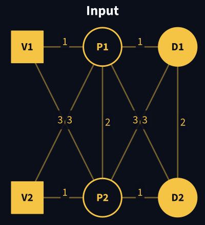
Figure 38: Two vehicles (V1, V2) and two requests (P1->D1, P2->D2) on a simple network with Manhattan edge costs.

Problem Instance

Network structure:

• 2 vehicle starts:
  • V1 at position (0, 2) (top-left), and
  • V2 at position (0, 0) (bottom-left).
• 2 requests:
  • \((P_1, D_1)\), and
  • \((P_2, D_2)\).
• Edge costs: Manhattan travel time on the layout (e.g., \(d(V1,P1)=1\), \(d(V1,P2)=3\), \(d(P1,D2)=3\)).

KPI dashboard:

Table 29: Metrics used to compare routes in this toy PDP instance.

Symbol	Meaning	Units
f_dist	Total distance traveled	distance units
f_wait	Pickup waiting + in-ride delay1	time units
SR	Service rate (= served customers / total customers)	%
f_fleet	Active vehicles used	count

\(SR = \frac{N_{\text{served}}}{N_{\text{customers}}} \times 100\).

Direct Path Baselines

• Request 1 direct leg: \(P_1 \to D_1\).
• Request 2 direct leg: \(P_2 \to D_2\).

1. Ride delay: Deviation from direct travel time.

Service Quality vs. Fleet Utilization Trade-off

Assuming we want to serve all customers:

1. If you maximize fleet utilization, one vehicle can serve both requests (see Figure 39). One pickup waits longer.
2. If you minimize total waiting time, each vehicle serves one request (see Figure 40). Fleet usage increases.

Figure 39: Minimizing total fleet size on the all-served feasible set.

Figure 40: Minimizing total waiting time on the all-served feasible set.

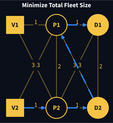
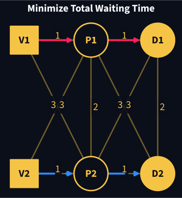
All Candidate Solutions Enumerated

Complete enumeration of candidate routing plans with KPI values in Table 30.

Enumeration Method

We enumerate every feasible combination by:

1. Assigning each request to V1, V2, or reject.
2. Generating all pickup/dropoff event orders that satisfy pickup-before-delivery.
3. Combining both vehicle routes and evaluating KPIs with Manhattan travel.

Table 30: Complete solution space for the ridesharing instance. Pareto-optimal solutions are marked in the Pareto column.

	ID	Routes	f_dist	f_wait	SR (%)	f_fleet	rejected	Pareto
0	S0	V1=() / V2=()	0	0	0	0	2	No
1	S1	V1=() / V2=(2,2')	2	1	50	1	1	No
2	S2	V1=(1,1') / V2=()	2	1	50	1	1	No
3	S3	V1=(1,1') / V2=(2,2')	4	2	100	2	0	Yes
4	S4	V1=() / V2=(1,1')	4	3	50	1	1	No
5	S5	V1=(2,2') / V2=()	4	3	50	1	1	No
6	S6	V1=() / V2=(2,1,1',2')	6	8	100	1	0	No
7	S7	V1=(1,2,2',1') / V2=()	6	8	100	1	0	No
8	S8	V1=() / V2=(2,2',1,1')	6	6	100	1	0	Yes
9	S9	V1=(1,1',2,2') / V2=()	6	6	100	1	0	Yes
10	S10	V1=() / V2=(2,1,2',1')	8	12	100	1	0	No
11	S11	V1=(1,2,1',2') / V2=()	8	12	100	1	0	No
12	S12	V1=(2,2') / V2=(1,1')	8	6	100	2	0	No
13	S13	V1=() / V2=(1,2,2',1')	8	12	100	1	0	No
14	S14	V1=(2,1,1',2') / V2=()	8	12	100	1	0	No
15	S15	V1=() / V2=(1,1',2,2')	8	10	100	1	0	No
16	S16	V1=(2,2',1,1') / V2=()	8	10	100	1	0	No
17	S17	V1=() / V2=(1,2,1',2')	10	16	100	1	0	No
18	S18	V1=(2,1,2',1') / V2=()	10	16	100	1	0	No

Candidate Solution Panel

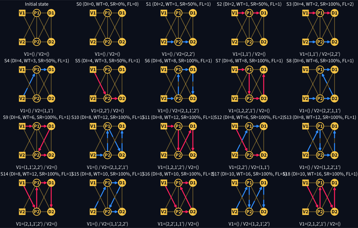
Figure 41: All candidate solutions on the toy PDP layout (V1, V2, P1, P2, D1, D2), including reject-all option S0. Route encoding uses V1=(1,1',2,2'); title labels are DI, WT, SR, and FL.

Key Observations

• Full enumeration yields 19 candidates for 2 vehicles and 2 requests.
• S0 is the reject-all option (V1=() / V2=()) with SR=0%.
• The enumerator covers all assignment patterns: V1-only, V2-only, split, and cross assignments.
• Optimization methods below use only all-served plans (rejected = 0).
• Under this all-served filter, every selectable plan has SR=100% by definition (served / total).
• Pareto-optimal and dominated plans are identified directly from the generated KPI table under this all-served feasibility filter.
• The fleet objective has a small numeric range, so weight scaling matters.

What is Pareto Optimality?

Formal definition (Geoffrion 1968; Caramia and Dell’Olmo 2008):

A solution \(\mathbf{x}^* \in S\) is Pareto optimal if there does not exist another \(\mathbf{x} \in S\) such that:

\[ f_i(\mathbf{x}) \leq f_i(\mathbf{x}^*) \quad \forall i \]

with at least one strict inequality:

\[ f_j(\mathbf{x}) < f_j(\mathbf{x}^*) \quad \text{for some } j \]

Pareto Dominance: Example

Consider one automatically detected dominance pair from Table 30. Table Table 31 compares their objective values.

Analysis: The dominating solution is no worse in all objectives and strictly better in at least one objective.

Figure 42: Geometric view in \((f_{\text{dist}}, f_{\text{wait}})\) space for the detected dominance pair.

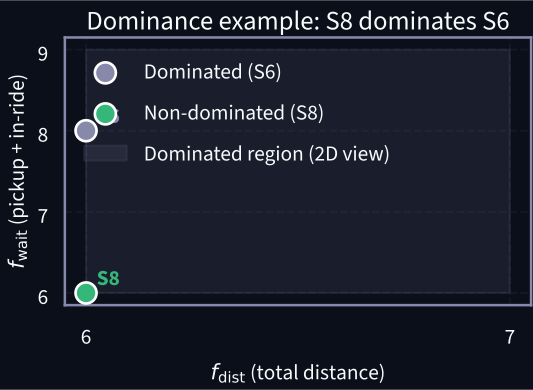
Figure 42: Geometric view in \((f_{\text{dist}}, f_{\text{wait}})\) space for the detected dominance pair.

Pareto Front Visualization

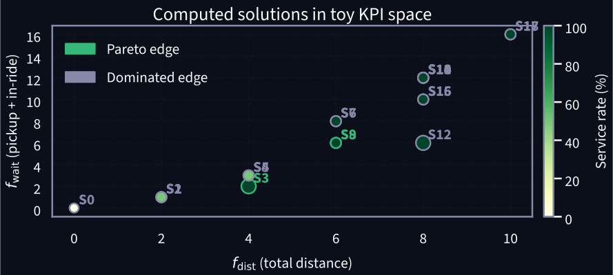
Figure 43: Toy KPI projection: distance vs total waiting. Color shows service rate and marker size shows fleet size.

2D Projection

This plot uses \((f_{\text{dist}}, f_{\text{wait}})\). Marker color encodes service rate and marker size encodes fleet size. The full front is still in 4D objective space. All candidate solutions are shown; Pareto status is indicated by marker edge color.

Non-Convex Pareto Front

This projection is non-convex. Weighted-sum scalarization may miss valid Pareto points (Chang 2015, sec. 5.3.2.1).

Criterion Space vs Design Space

Design space (decision variables):

• Vehicle-customer assignments
• Route sequences
• Timing decisions

For our instance, Table 30 lists all enumerated candidate plans, including V1-only, V2-only, split, cross, and reject-all cases.

Each routing plan \(\mathbf{x}\) maps to a point in criterion space via the objective functions:

\[ \mathbf{x} \xrightarrow{f} \mathbf{z} = (f_{\text{dist}}, f_{\text{wait}}, SR, f_{\text{fleet}}) \]

graph LR
    subgraph "Design Space (Enumerated Routes)"
        XA["Route A<br>V1=(...)<br>V2=(...)"]
        XB["Route B<br>V1=(...)<br>V2=(...)"]
        XC["Route C<br>V1=(...)<br>V2=(...)"]
        X0["Reject-all<br>V1=()<br>V2=()"]
    end
    subgraph "Criterion Space (4D)"
        ZA["(f_dist, f_wait, SR, f_fleet)"]
        ZB["(f_dist, f_wait, SR, f_fleet)"]
        ZC["(f_dist, f_wait, SR, f_fleet)"]
        Z0["(0, high, 0, 0)"]
    end
    XA -- "f( )" --> ZA
    XB -- "f( )" --> ZB
    XC -- "f( )" --> ZC
    X0 -- "f( )" --> Z0

    style ZA fill:#35b779
    style ZB fill:#35b779
    style ZC fill:#35b779
    style Z0 fill:#8888aa

Figure 44: Design space (routes) vs criterion space (objectives). Different routing plans map to points in 4D objective space.

Example: Two routes can have similar distance but different waiting, service rate, and fleet trade-offs.

Formal Multi-Objective Statement

The ridesharing problem seeks to optimize four objectives simultaneously:

\[ \min \left[ f_{\text{dist}}(\mathbf{x}), f_{\text{wait}}(\mathbf{x}), f_{\text{fleet}}(\mathbf{x}) \right], \quad \max \ SR(\mathbf{x}) \]

subject to:

\[ \mathbf{x} \in S \]

where \(S\) is the set of service-feasible routing plans (vehicle capacity, time windows, pickup-before-delivery, etc.) with all requests served (n_rejected = 0). In this deck, S0 is shown only as a policy fallback benchmark, not as a selectable optimization solution.

Service rate is defined as:

\[ SR(\mathbf{x}) = \frac{N_{\text{served}}(\mathbf{x})}{N_{\text{customers}}} \times 100 \]

so, over the all-served feasible set \(S\), \(SR(\mathbf{x}) = 100\%\) for every selectable solution.

Solution Concept

The goal is to find the Pareto-optimal set—the collection of all non-dominated solutions. Decision-makers then select from this set based on preferences (Caramia and Dell’Olmo 2008).

Why Normalization Matters

In the full candidate space, objectives have different units and scales. In the all-served selectable set, SR is fixed at 100% (see Table 32):

Table 32: Objective value ranges across selectable solutions.

	Objective	Min	Max	Range	Best solutions
0	f_dist	4	10	6	S3
1	f_wait	2	16	14	S3
2	SR (%)	100	100	0	S3, S6, S7, S8, S9, S10, ...
3	f_fleet	1	2	1	S6, S7, S8, S9, S10, S11, ...

Observation: In this mandatory-service subset, SR has zero range (100% for all selectable plans). In broader instances where rejection is allowed, normalization remains important before applying weighted methods.

Impact on Weighted Sum

Without normalization, the widest-range objective can dominate weighted-sum scores regardless of stakeholder intent.

Weights reflect both user preferences AND scale differences (Arora 2017, sec. 18.2.6).

For simplicity, our discrete problem uses integer weights as priorities rather than normalized weights. Real-world continuous problems should normalize objectives to \([0,1]\) first.

Normalization Formula

\[f_i^{\text{norm}}(\mathbf{x}) = \frac{f_i(\mathbf{x}) - f_i^{\min}}{f_i^{\max} - f_i^{\min}}\]

Solution Techniques Overview

Since there are multiple Pareto-optimal solutions, we need methods to:

1. Incorporate decision-maker preferences to select a single solution
2. Generate representative Pareto sets for visualization and exploration

Table Table 33 summarizes the main choices.

Table 33: Comparison of multi-objective solution techniques.

Method	Preference input	Finds all Pareto points?
Weighted sum	Objective weights W_k	No (only convex parts)
Epsilon-constraints	Budget limits epsilon_k	Yes (with parameter sweep)
Goal programming	Target values T_k	No (minimizes deviations)
Lexicographic	Priority ordering	No (one point per ordering)

Method Selection Strategy

• Exploring trade-offs: Use \(\varepsilon\)-constraints to generate the full Pareto set, then visualize
• Known preferences: Use weighted sum or goal programming
• Clear priority order: Use lexicographic method

Weighted Sum

Method 1

Preference-weighted scalarization of multiple objectives

01

Weighted Sum: Concept

Idea: Combine multiple objectives into a single scalar function using weights.

\[ \min \sum_{k=1}^{n} w_k \cdot f_k(\mathbf{x}) \]

subject to:

\[ \sum_{k=1}^{n} w_k = 1, \quad w_k > 0, \quad \mathbf{x} \in S \]

Geometric interpretation (2D case): Find the point on the Pareto front where a line with slope \(-\frac{w_1}{w_2}\) is tangent to the feasible region.

Figure 45: Weighted sum sweeps a line across criterion space. Different weight vectors \(\mathbf{w}\) find different supported Pareto points. The non-convex point is not selected.

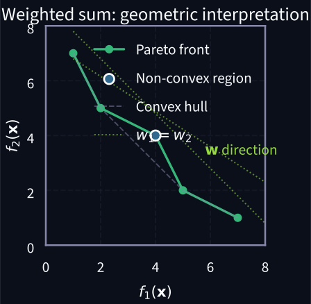
Mathematical Formulation

For our discrete ridesharing problem with pre-enumerated solutions, we select one solution by minimizing a weighted combination of its objectives.

Decision variables:

\[ z_s \in \{0, 1\}, \quad s \in \text{Solutions} \]

where \(z_s = 1\) if solution \(s\) is selected, 0 otherwise.

Weighted-sum formulation:

\[ \min \sum_{s \in \text{Solutions}} \left( \sum_{k} W_k \cdot f_k^s \right) z_s \]

subject to:

\[ \sum_{s \in \text{Solutions}} z_s = 1 \quad \text{(select exactly one solution)} \]

\[ z_s \in \{0, 1\}, \quad \forall s \]

where \(W_k \in \mathbb{Z}_{>0}\) are integer priority weights and \(f_k^s\) is the value of objective \(k\) for solution \(s\).

Implementation and Results

Listing 10: Weighted-sum method: minimize a weighted combination of objectives. Integer weights avoid fractional arithmetic.

def weighted_sum_select(
    weights: dict[str, int]
) -> tuple[str, int]:
    """
    Select solution minimizing weighted objective sum.

    Args:
        weights: Priority weights for each objective
                 (dist, wait, service, fleet)

    Returns:
        (selected_solution_id, weighted_objective_value)
    """
    # Create optimization problem
    prob = LpProblem("MO_WeightedSum", LpMinimize)

    # Binary variable: z[s] = 1 if solution s selected
    z = LpVariable.dicts(
        "z",
        list(solutions),
        cat="Binary"
    )

    # Objective: weighted sum of all objectives
    prob += lpSum(
        (
            weights["dist"] * solutions[sid]["f_dist"]
            + weights["wait"] * solutions[sid]["f_wait"]
            + weights["service"] * (100 - solutions[sid]["service_rate"])
            + weights["fleet"] * solutions[sid]["f_fleet"]
        )
        * z[sid]
        for sid in solutions
    )

    # Constraint: select exactly one solution
    prob += lpSum(z[sid] for sid in solutions) == 1

    # Solve
    prob.solve(PULP_CBC_CMD(msg=0))

    # Extract selected solution
    selected = next(
        sid for sid in solutions
        if value(z[sid]) > 0.5
    )

    return selected, int(round(value(prob.objective)))

Listing 11: Results for three different weight configurations. Changing weights explores different Pareto-optimal trade-offs.

# Test different priority configurations
priority_sets = {
    "Distance priority": {
        "dist": 7,
        "wait": 2,
        "service": 4,
        "fleet": 3
    },
    "Waiting priority": {
        "dist": 2,
        "wait": 7,
        "service": 3,
        "fleet": 3
    },
    "Service priority": {
        "dist": 2,
        "wait": 2,
        "service": 8,
        "fleet": 3
    },
    "Fleet priority": {
        "dist": 2,
        "wait": 2,
        "service": 3,
        "fleet": 7,
    },
}

for name, weights in priority_sets.items():
    sid, obj = weighted_sum_select(weights)
    vals = objective_tuple(sid)
    print(f"{name}:")
    print(f"  Solution: {sid}")
    print(
        f"  dist={vals[0]}, wait={vals[1]}, "
        f"SR={vals[2]}%, fleet={vals[3]}"
    )
    print(f"  Weighted score: {obj}\n")

Distance priority:
  Solution: S3
  dist=4, wait=2, SR=100%, fleet=2
  Weighted score: 38

Waiting priority:
  Solution: S3
  dist=4, wait=2, SR=100%, fleet=2
  Weighted score: 28

Service priority:
  Solution: S3
  dist=4, wait=2, SR=100%, fleet=2
  Weighted score: 18

Fleet priority:
  Solution: S3
  dist=4, wait=2, SR=100%, fleet=2
  Weighted score: 26

Weighted Sum: Limitation

Non-Convex Pareto Fronts Cannot Be Fully Explored

Theorem (Geoffrion 1968): If the solution set \(S\) is convex and the objectives \(f_i\) are convex, then the weighted-sum method finds strict Pareto optima for any \(w_i > 0\).

Limitation: If the Pareto front is non-convex, some Pareto-optimal points are not minimizers for any choice of weights (Chang 2015, sec. 5.3.2.1; Arora 2017, sec. 18.4).

Figure 46: Non-convex Pareto front (black curve). Weighted sum selects supported points on the convex hull and misses the unsupported point.

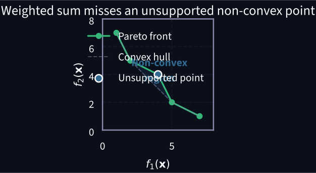
Implication for this ridesharing dataset:

The Pareto front in Figure 43 shows non-convex sections.

Consequence: Systematic weight sweeps can miss valid Pareto-optimal points.

Alternative: Use \(\varepsilon\)-constraints (Method 2) to recover the full front.

Convex vs Non-Convex Pareto Fronts

A Pareto front is convex if every point lies on the convex hull of the objective space.

Non-convex fronts have points that lie inside (above) the convex hull — a “dent” in the front.

Why non-convexity arises:

• Discrete / integer variables
• Non-convex objective functions
• Combinatorial structure (routing, scheduling)
• Mixed-integer programs

Key consequence: Weighted-sum methods can only find points on the convex hull — they skip unsupported non-convex points.

* Convex hull: the smallest convex shape enclosing all Pareto points — imagine stretching a rubber band around them.

{
  async function loadThemeConfigCvx() {
    const paths = [
      "/config/graphics-colors.json",
      "../config/graphics-colors.json",
      "config/graphics-colors.json",
    ];
    for (const path of paths) {
      try {
        const response = await fetch(path);
        if (response.ok) {
          return await response.json();
        }
      } catch (error) {
        // Continue to the next path candidate.
      }
    }
    throw new Error("Could not load config/graphics-colors.json");
  }

  function hexToRgbaCvx(hexColor, alpha) {
    const clean = hexColor.replace("#", "").trim();
    const expanded = clean.length === 3
      ? clean.split("").map((char) => char + char).join("")
      : clean;
    const value = Number.parseInt(expanded, 16);
    if (Number.isNaN(value) || expanded.length !== 6) {
      return `rgba(255, 255, 255, ${alpha})`;
    }
    const red = (value >> 16) & 255;
    const green = (value >> 8) & 255;
    const blue = value & 255;
    return `rgba(${red}, ${green}, ${blue}, ${alpha})`;
  }

  const themeConfigCvx = await loadThemeConfigCvx();
  const selectedThemeCvx = (
    window.GRAPHICS_THEME ??
    window.SLIDE_THEME ??
    themeConfigCvx.default_theme
  );
  const themeCvx = (
    themeConfigCvx.themes[selectedThemeCvx] ??
    themeConfigCvx.themes[themeConfigCvx.default_theme]
  );
  const fontConfigCvx = themeConfigCvx.font ?? {};
  const BG = themeCvx.background;
  const PARETO = themeCvx.primary;
  const ACCENT = themeCvx.accent;
  const SECONDARY = themeCvx.secondary;
  const ERROR = themeCvx.error;
  const TEXT = themeCvx.text_primary;
  const GRID = themeCvx.grid;
  const STROKE = themeCvx.white;
  const FONT = (
    fontConfigCvx.ojs_css_stack ??
    '"Source Sans 3", "Inter", "Segoe UI", "DejaVu Sans", "Arial", sans-serif'
  );

  const totalW = 920, totalH = 560;
  const panelW = 420, panelH = 440;
  const gap = 80;
  const margin = { top: 60, right: 30, bottom: 55, left: 55 };
  const panelInnerW = panelW - margin.left - margin.right;
  const panelInnerH = panelH - margin.top - margin.bottom;
  const iSize = Math.min(panelInnerW, panelInnerH);
  const iW = iSize;
  const iH = iSize;
  const plotOffsetX = (panelInnerW - iW) / 2;

  // Minimal 5-point teaching example.
  // Convex front: every point is supported.
  const convF1 = [1, 2, 3, 5, 7];
  const convF2 = [7, 5, 3, 2, 1];

  // Non-convex front: (4, 4) is the single unsupported Pareto point.
  const ncF1 = [1, 2, 4, 5, 7];
  const ncF2 = [7, 5, 4, 2, 1];

  // Convex hull of the non-convex front (skips x = 4).
  const hullF1 = [1, 2, 5, 7];
  const hullF2 = [7, 5, 2, 1];

  const container = d3.create("div").style("position", "relative");
  const svg = container.append("svg")
    .attr("viewBox", `0 0 ${totalW} ${totalH}`)
    .style("max-width", "100%").style("height", "auto")
    .style("background", BG).style("border-radius", "8px")
    .style("font-family", FONT);

  function drawPanel(xOff, title, f1Arr, f2Arr, isNonConvex) {
    const panel = svg.append("g").attr("transform", `translate(${xOff}, 0)`);
    const g = panel.append("g").attr(
      "transform",
      `translate(${margin.left + plotOffsetX},${margin.top})`
    );

    const x = d3.scaleLinear().domain([0, 8]).range([0, iW]);
    const y = d3.scaleLinear().domain([0, 8]).range([iH, 0]);

    // Grid
    for (let i = 1; i <= 7; i += 1) {
      g.append("line").attr("x1", x(i)).attr("x2", x(i)).attr("y1", 0).attr("y2", iH)
        .attr("stroke", GRID).attr("stroke-dasharray", "2,4").attr("opacity", 0.4);
      g.append("line").attr("x1", 0).attr("x2", iW).attr("y1", y(i)).attr("y2", y(i))
        .attr("stroke", GRID).attr("stroke-dasharray", "2,4").attr("opacity", 0.4);
    }

    // Axes
    g.append("g").attr("transform", `translate(0,${iH})`).call(d3.axisBottom(x).ticks(6))
      .call(g => g.selectAll("text").attr("fill", TEXT).style("font-size", "12px"))
      .call(g => g.selectAll("line,path").attr("stroke", TEXT).attr("opacity", 0.5));
    g.append("g").call(d3.axisLeft(y).ticks(6))
      .call(g => g.selectAll("text").attr("fill", TEXT).style("font-size", "12px"))
      .call(g => g.selectAll("line,path").attr("stroke", TEXT).attr("opacity", 0.5));
    g.append("text").attr("x", iW / 2).attr("y", iH + 42).attr("text-anchor", "middle")
      .attr("fill", TEXT).style("font-size", "13px").text("f\u2081(x)");
    g.append("text").attr("transform", "rotate(-90)").attr("x", -iH / 2).attr("y", -40)
      .attr("text-anchor", "middle").attr("fill", TEXT).style("font-size", "13px").text("f\u2082(x)");

    // Title
    panel.append("text").attr("x", margin.left + plotOffsetX + iW / 2).attr("y", 25)
      .attr("text-anchor", "middle").attr("fill", TEXT)
      .style("font-size", "16px").style("font-weight", "600").text(title);

    const data = f1Arr.map((f1, i) => ({ f1, f2: f2Arr[i] }));
    const line = d3.line().x(d => x(d.f1)).y(d => y(d.f2)).curve(d3.curveMonotoneX);

    // Dynamic layer for animation
    const dynLayer = g.append("g");

    // Pareto front
    g.append("path").datum(data).attr("d", line)
      .attr("fill", "none").attr("stroke", PARETO).attr("stroke-width", 2.5);
    const dots = g.selectAll(".pt").data(data).join("circle")
      .attr("cx", d => x(d.f1)).attr("cy", d => y(d.f2))
      .attr("r", 5).attr("fill", PARETO).attr("stroke", STROKE).attr("stroke-width", 1);

    if (isNonConvex) {
      // Non-convex point to highlight
      const ncPoints = data.filter(d => d.f1 === 4);
      const ncDots = g.selectAll(".nc").data(ncPoints).join("circle")
        .attr("cx", d => x(d.f1)).attr("cy", d => y(d.f2))
        .attr("r", 7).attr("fill", "none").attr("stroke", ACCENT)
        .attr("stroke-width", 2.5).attr("opacity", 0);

      // Convex hull dashed line — bright white for visibility
      const hullData = hullF1.map((f1, i) => ({ f1, f2: hullF2[i] }));
      const hullLine = d3.line().x(d => x(d.f1)).y(d => y(d.f2));
      const hullPath = g.append("path").datum(hullData).attr("d", hullLine)
        .attr("fill", "none").attr("stroke", STROKE)
        .attr("stroke-width", 2.5).attr("stroke-dasharray", "10,6").attr("opacity", 0);

      // Shaded gap area between hull and front
      const gapArea = g.append("path")
        .attr("d", `M${x(2)},${y(5)} L${x(5)},${y(2)} L${x(4)},${y(4)} Z`)
        .attr("fill", ERROR).attr("opacity", 0);

      // Label
      const gapLabel = g.append("text")
        .attr("x", x(4.1)).attr("y", y(3.45)).attr("text-anchor", "middle")
        .attr("fill", ERROR).style("font-size", "12px").style("font-weight", "600")
        .attr("opacity", 0).text("Gap: missed by weighted sum");

      // Result label
      const resultLabel = panel.append("text")
        .attr("x", margin.left + plotOffsetX + iW / 2).attr("y", panelH - 5)
        .attr("text-anchor", "middle").attr("fill", ERROR)
        .style("font-size", "14px").style("font-weight", "600")
        .attr("opacity", 0).text("Non-convex: gap between hull and front \u2717");

      return { hullPath, gapArea, gapLabel, ncDots, resultLabel };
    } else {
      // For convex: hull IS the front — bright white for visibility
      const hullPath = g.append("path").datum(data)
        .attr("d", d3.line().x(d => x(d.f1)).y(d => y(d.f2)))
        .attr("fill", "none").attr("stroke", STROKE)
        .attr("stroke-width", 2.5).attr("stroke-dasharray", "10,6").attr("opacity", 0);

      const resultLabel = panel.append("text")
        .attr("x", margin.left + plotOffsetX + iW / 2).attr("y", panelH - 5)
        .attr("text-anchor", "middle").attr("fill", PARETO)
        .style("font-size", "14px").style("font-weight", "600")
        .attr("opacity", 0).text("Convex: every point reachable \u2713");

      return { hullPath, resultLabel };
    }
  }

  const leftPanel = drawPanel(0, "Convex Pareto Front", convF1, convF2, false);
  const rightPanel = drawPanel(panelW + gap, "Non-Convex Pareto Front", ncF1, ncF2, true);

  const delay = ms => new Promise(r => setTimeout(r, ms));

  async function animate() {
    // Reset
    leftPanel.hullPath.attr("opacity", 0);
    leftPanel.resultLabel.attr("opacity", 0);
    rightPanel.hullPath.attr("opacity", 0);
    rightPanel.gapArea.attr("opacity", 0);
    rightPanel.gapLabel.attr("opacity", 0);
    rightPanel.ncDots.attr("opacity", 0);
    rightPanel.resultLabel.attr("opacity", 0);

    await delay(800);

    // Step 1: Draw convex hulls on both
    leftPanel.hullPath.transition().duration(800).attr("opacity", 0.7);
    rightPanel.hullPath.transition().duration(800).attr("opacity", 0.7);
    await delay(1200);

    // Step 2: Show gap on non-convex
    rightPanel.gapArea.transition().duration(600).attr("opacity", 0.15);
    await delay(400);
    rightPanel.ncDots.transition().duration(400).attr("opacity", 1);
    await delay(400);
    rightPanel.gapLabel.transition().duration(400).attr("opacity", 1);
    await delay(1000);

    // Step 3: Show result labels
    leftPanel.resultLabel.transition().duration(400).attr("opacity", 1);
    rightPanel.resultLabel.transition().duration(400).attr("opacity", 1);
  }

  // Legend
  const leg = svg.append("g").attr("transform", `translate(${totalW / 2 - 180}, ${totalH - 20})`);
  leg.append("line").attr("x1", 0).attr("x2", 20).attr("y1", 0).attr("y2", 0)
    .attr("stroke", PARETO).attr("stroke-width", 2.5);
  leg.append("circle").attr("cx", 10).attr("cy", 0).attr("r", 4)
    .attr("fill", PARETO).attr("stroke", STROKE).attr("stroke-width", 1);
  leg.append("text").attr("x", 26).attr("y", 1).attr("fill", TEXT)
    .attr("dominant-baseline", "middle").style("font-size", "12px").text("Pareto front");
  leg.append("line").attr("x1", 130).attr("x2", 150).attr("y1", 0).attr("y2", 0)
    .attr("stroke", STROKE).attr("stroke-width", 2.5).attr("stroke-dasharray", "10,6");
  leg.append("text").attr("x", 156).attr("y", 1).attr("fill", TEXT)
    .attr("dominant-baseline", "middle").style("font-size", "12px").text("Convex hull*");
  leg.append("circle").attr("cx", 270).attr("cy", 0).attr("r", 6)
    .attr("fill", "none").attr("stroke", ACCENT).attr("stroke-width", 2);
  leg.append("text").attr("x", 282).attr("y", 1).attr("fill", TEXT)
    .attr("dominant-baseline", "middle").style("font-size", "12px").text("Non-convex point");

  const BUTTON_BG = hexToRgbaCvx(STROKE, 0.12);
  const BUTTON_BORDER = hexToRgbaCvx(STROKE, 0.25);
  container.append("button").text("\u25b6 Replay")
    .style("position", "absolute").style("top", "8px").style("left", "8px")
    .style("background", BUTTON_BG).style("color", TEXT)
    .style("border", `1px solid ${BUTTON_BORDER}`).style("border-radius", "4px")
    .style("padding", "4px 12px").style("cursor", "pointer")
    .style("font-family", FONT).style("font-size", "13px")
    .on("click", () => animate());

  const node = container.node();
  const obs = new IntersectionObserver((entries) => {
    if (entries[0].isIntersecting) { animate(); obs.disconnect(); }
  }, { threshold: 0.3 });
  requestAnimationFrame(() => obs.observe(node));

  yield node;
}

Figure 47

Weighted Sum: Why It Fails on Non-Convex Fronts

Geometric insight: The weighted sum \(\min(w_1 f_1 + w_2 f_2)\) finds where an iso-cost line is tangent to the Pareto front.

On a convex front, every point is tangent for some weight ratio — all points are reachable.

On a non-convex front, the tangent line jumps over the concavity; some Pareto points are not minimizers for any weighted sum.

The iso-cost line sweeps from vertical (\(w_1 \gg w_2\)) to horizontal (\(w_2 \gg w_1\)), and the tangent point traces only the convex hull.

A line through a Pareto point does not guarantee selection; weighted sum picks the lowest parallel line of that slope.

For a fixed ratio \(r = w_1 / w_2\), define \(z(x) = r f_1(x) + f_2(x)\). Weighted sum selects the point with minimum \(z(x)\).

{
  async function loadThemeConfigWs() {
    const paths = [
      "/config/graphics-colors.json",
      "../config/graphics-colors.json",
      "config/graphics-colors.json",
    ];
    for (const path of paths) {
      try {
        const response = await fetch(path);
        if (response.ok) {
          return await response.json();
        }
      } catch (error) {
        // Continue to the next path candidate.
      }
    }
    throw new Error("Could not load config/graphics-colors.json");
  }

  function hexToRgbaWs(hexColor, alpha) {
    const clean = hexColor.replace("#", "").trim();
    const expanded = clean.length === 3
      ? clean.split("").map((char) => char + char).join("")
      : clean;
    const value = Number.parseInt(expanded, 16);
    if (Number.isNaN(value) || expanded.length !== 6) {
      return `rgba(255, 255, 255, ${alpha})`;
    }
    const red = (value >> 16) & 255;
    const green = (value >> 8) & 255;
    const blue = value & 255;
    return `rgba(${red}, ${green}, ${blue}, ${alpha})`;
  }

  const themeConfigWs = await loadThemeConfigWs();
  const selectedThemeWs = (
    window.GRAPHICS_THEME ??
    window.SLIDE_THEME ??
    themeConfigWs.default_theme
  );
  const themeWs = (
    themeConfigWs.themes[selectedThemeWs] ??
    themeConfigWs.themes[themeConfigWs.default_theme]
  );
  const fontConfigWs = themeConfigWs.font ?? {};
  const BG = themeWs.background;
  const PARETO = themeWs.primary;
  const ACCENT = themeWs.accent;
  const SECONDARY = themeWs.secondary;
  const ERROR = themeWs.error;
  const TEXT = themeWs.text_primary;
  const GRID = themeWs.grid;
  const STROKE = themeWs.white;
  const FONT = (
    fontConfigWs.ojs_css_stack ??
    '"Source Sans 3", "Inter", "Segoe UI", "DejaVu Sans", "Arial", sans-serif'
  );
  const CANDIDATE_LINE = hexToRgbaWs(TEXT, 0.78);
  const totalW = 760, totalH = 680;
  const margin = { top: 54, right: 34, bottom: 84, left: 52 };
  const plotBaseW = totalW - margin.left - margin.right;
  const plotBaseH = totalH - margin.top - margin.bottom;
  const iSize = Math.min(plotBaseW, plotBaseH);
  const iW = iSize;
  const iH = iSize;
  const plotLeft = margin.left + (plotBaseW - iW) / 2;

  // Non-convex front with one unsupported middle point.
  const ncF1 = [1, 2, 4, 5, 7];
  const ncF2 = [7, 5, 4, 2, 1];
  const ncData = ncF1.map((f1, i) => ({ f1, f2: ncF2[i] }));
  const unsupportedIndices = [2]; // (4, 4)

  const container = d3.create("div").style("position", "relative");
  const svg = container.append("svg")
    .attr("viewBox", `0 0 ${totalW} ${totalH}`)
    .style("max-width", "100%").style("height", "auto")
    .style("background", BG).style("border-radius", "8px")
    .style("font-family", FONT);

  // Weight steps: w1/(w1+w2) from 0.02 to 0.98
  const weightSteps = [];
  for (let r = 0.02; r <= 0.98; r += 0.02) weightSteps.push(r);

  function findTangentPoint(data, w1, w2) {
    let best = null, bestVal = Infinity;
    for (const d of data) {
      const val = w1 * d.f1 + w2 * d.f2;
      if (val < bestVal) { bestVal = val; best = d; }
    }
    return { point: best, cost: bestVal };
  }

  function lineSegmentForCost(w1, w2, cost) {
    const xMin = 0;
    const xMax = 8;
    const yMin = 0;
    const yMax = 8;
    const eps = 1e-9;
    const pts = [];

    function addPoint(px, py) {
      if (px < xMin - eps || px > xMax + eps || py < yMin - eps || py > yMax + eps) {
        return;
      }
      const xClamped = Math.max(xMin, Math.min(xMax, px));
      const yClamped = Math.max(yMin, Math.min(yMax, py));
      for (const p of pts) {
        if (Math.abs(p.x - xClamped) < 1e-6 && Math.abs(p.y - yClamped) < 1e-6) {
          return;
        }
      }
      pts.push({ x: xClamped, y: yClamped });
    }

    if (Math.abs(w2) > eps) {
      addPoint(xMin, (cost - w1 * xMin) / w2);
      addPoint(xMax, (cost - w1 * xMax) / w2);
    }
    if (Math.abs(w1) > eps) {
      addPoint((cost - w2 * yMin) / w1, yMin);
      addPoint((cost - w2 * yMax) / w1, yMax);
    }

    if (pts.length < 2) {
      return { x1: xMin, y1: yMin, x2: xMax, y2: yMax };
    }

    let a = pts[0];
    let b = pts[1];
    let bestD2 = -1;
    for (let i = 0; i < pts.length; i += 1) {
      for (let j = i + 1; j < pts.length; j += 1) {
        const dx = pts[i].x - pts[j].x;
        const dy = pts[i].y - pts[j].y;
        const d2 = dx * dx + dy * dy;
        if (d2 > bestD2) {
          bestD2 = d2;
          a = pts[i];
          b = pts[j];
        }
      }
    }

    return { x1: a.x, y1: a.y, x2: b.x, y2: b.y };
  }

  function lineSegmentThroughPoint(w1, w2, point) {
    const anchoredCost = w1 * point.f1 + w2 * point.f2;
    return lineSegmentForCost(w1, w2, anchoredCost);
  }

  const g = svg.append("g").attr("transform", `translate(${plotLeft},${margin.top})`);
  const x = d3.scaleLinear().domain([0, 8]).range([0, iW]);
  const y = d3.scaleLinear().domain([0, 8]).range([iH, 0]);

  for (let i = 1; i <= 7; i += 1) {
    g.append("line").attr("x1", x(i)).attr("x2", x(i)).attr("y1", 0).attr("y2", iH)
      .attr("stroke", GRID).attr("stroke-dasharray", "2,4").attr("opacity", 0.4);
    g.append("line").attr("x1", 0).attr("x2", iW).attr("y1", y(i)).attr("y2", y(i))
      .attr("stroke", GRID).attr("stroke-dasharray", "2,4").attr("opacity", 0.4);
  }
  g.append("g").attr("transform", `translate(0,${iH})`).call(d3.axisBottom(x).ticks(8))
    .call(g => g.selectAll("text").attr("fill", TEXT).style("font-size", "12px"))
    .call(g => g.selectAll("line,path").attr("stroke", TEXT).attr("opacity", 0.5));
  g.append("g").call(d3.axisLeft(y).ticks(8))
    .call(g => g.selectAll("text").attr("fill", TEXT).style("font-size", "12px"))
    .call(g => g.selectAll("line,path").attr("stroke", TEXT).attr("opacity", 0.5));
  g.append("text").attr("x", iW / 2).attr("y", iH + 44).attr("text-anchor", "middle")
    .attr("fill", TEXT).style("font-size", "14px").text("f\u2081(x)");
  g.append("text").attr("transform", "rotate(-90)").attr("x", -iH / 2).attr("y", -45)
    .attr("text-anchor", "middle").attr("fill", TEXT).style("font-size", "14px").text("f\u2082(x)");

  svg.append("text")
    .attr("x", plotLeft + iW / 2).attr("y", 26)
    .attr("text-anchor", "middle").attr("fill", TEXT)
    .style("font-size", "16px").style("font-weight", "600")
    .text("Non-Convex Front");

  const frontLine = d3.line().x(d => x(d.f1)).y(d => y(d.f2)).curve(d3.curveMonotoneX);
  g.append("path").datum(ncData).attr("d", frontLine)
    .attr("fill", "none").attr("stroke", PARETO).attr("stroke-width", 2.5);
  g.selectAll(".pt").data(ncData).join("circle")
    .attr("cx", d => x(d.f1)).attr("cy", d => y(d.f2))
    .attr("r", 5).attr("fill", PARETO).attr("stroke", STROKE).attr("stroke-width", 1);

  const isoLine = g.append("line")
    .attr("stroke", ACCENT).attr("stroke-width", 2).attr("opacity", 0);
  const tangentDot = g.append("circle")
    .attr("r", 9).attr("fill", SECONDARY).attr("stroke", STROKE)
    .attr("stroke-width", 2).attr("opacity", 0);
  const foundLayer = g.append("g");

  const explainLayer = g.append("g");
  const candidateLine = explainLayer.append("line")
    .attr("stroke", CANDIDATE_LINE).attr("stroke-width", 2.2)
    .attr("stroke-dasharray", "8,6").attr("opacity", 0);
  const winnerLine = explainLayer.append("line")
    .attr("stroke", ACCENT).attr("stroke-width", 2.8).attr("opacity", 0);
  const focusHalo = explainLayer.append("circle")
    .attr("r", 12).attr("fill", "none").attr("stroke", SECONDARY)
    .attr("stroke-width", 2.2).attr("stroke-dasharray", "4,4").attr("opacity", 0);
  const explainText = g.append("text")
    .attr("x", iW / 2).attr("y", iH - 12)
    .attr("text-anchor", "middle").attr("fill", TEXT)
    .style("font-size", "11px").style("font-weight", "600")
    .attr("opacity", 0);

  const weightLabel = svg.append("text")
    .attr("x", plotLeft + iW / 2).attr("y", 46)
    .attr("text-anchor", "middle").attr("fill", ACCENT)
    .style("font-size", "15px").style("font-weight", "600")
    .style("font-family", FONT).attr("opacity", 1);
  const counterText = svg.append("text")
    .attr("x", plotLeft + 8).attr("y", 68).attr("text-anchor", "start")
    .attr("fill", ACCENT).style("font-size", "14px").style("font-weight", "600")
    .attr("opacity", 1);

  const delay = ms => new Promise(r => setTimeout(r, ms));

  async function animate() {
    foundLayer.selectAll("*").remove();
    isoLine.interrupt().attr("opacity", 0);
    tangentDot.interrupt().attr("opacity", 0);
    candidateLine.interrupt().attr("opacity", 0);
    winnerLine.interrupt().attr("opacity", 0);
    focusHalo.interrupt().attr("opacity", 0);
    explainText.interrupt().attr("opacity", 0).text("");
    weightLabel.attr("opacity", 1).text("Sweep: r = w\u2081 / w\u2082");
    counterText.attr("fill", ACCENT).attr("opacity", 1).text("Found: 0/5");

    const found = new Set();
    await delay(500);

    for (const r of weightSteps) {
      const w1 = r;
      const w2 = 1 - r;
      weightLabel.text(`r = ${(w1 / w2).toFixed(2)} (w\u2081 / w\u2082)`);

      const { point } = findTangentPoint(ncData, w1, w2);
      const seg = lineSegmentThroughPoint(w1, w2, point);
      const lineTransition = isoLine.transition().duration(180).ease(d3.easeLinear)
        .attr("opacity", 0.62)
        .attr("x1", x(seg.x1)).attr("y1", y(seg.y1))
        .attr("x2", x(seg.x2)).attr("y2", y(seg.y2));
      const dotTransition = tangentDot.transition().duration(180).ease(d3.easeLinear)
        .attr("opacity", 1).attr("cx", x(point.f1)).attr("cy", y(point.f2));
      await Promise.all([lineTransition.end(), dotTransition.end()]);

      const key = `${point.f1},${point.f2}`;
      if (!found.has(key)) {
        found.add(key);
        foundLayer.append("circle")
          .attr("cx", x(point.f1)).attr("cy", y(point.f2))
          .attr("r", 0).attr("fill", SECONDARY).attr("stroke", STROKE).attr("stroke-width", 2)
          .transition().duration(260).ease(d3.easeBackOut).attr("r", 8);
      }
      counterText.text(`Found: ${found.size}/5`);
      await delay(60);
    }

    isoLine.transition().duration(260).attr("opacity", 0);
    tangentDot.transition().duration(260).attr("opacity", 0);
    weightLabel.text("Sweep complete. Test one fixed slope on the missed point.");
    await delay(600);

    for (const idx of unsupportedIndices) {
      const d = ncData[idx];
      if (!found.has(`${d.f1},${d.f2}`)) {
        const cx = x(d.f1);
        const cy = y(d.f2);
        const sz = 6;
        foundLayer.append("line")
          .attr("x1", cx - sz).attr("y1", cy - sz).attr("x2", cx + sz).attr("y2", cy + sz)
          .attr("stroke", ERROR).attr("stroke-width", 3).attr("opacity", 0)
          .transition().duration(300).attr("opacity", 1);
        foundLayer.append("line")
          .attr("x1", cx + sz).attr("y1", cy - sz).attr("x2", cx - sz).attr("y2", cy + sz)
          .attr("stroke", ERROR).attr("stroke-width", 3).attr("opacity", 0)
          .transition().duration(300).attr("opacity", 1);
      }
    }

    counterText.attr("fill", ERROR).text(`Found: ${found.size}/5 --- ${5 - found.size} missed!`);
    await delay(750);
    await counterText.transition().duration(220).attr("opacity", 0).end();

    const focusPoint = ncData[2]; // (4, 4)
    const winnerPoint = ncData[1]; // (2, 5)
    const rDemo = 1.2;
    const w1Demo = rDemo / (1 + rDemo);
    const w2Demo = 1 / (1 + rDemo);
    const candidateSeg = lineSegmentThroughPoint(w1Demo, w2Demo, focusPoint);
    const winnerSeg = lineSegmentThroughPoint(w1Demo, w2Demo, winnerPoint);

    weightLabel.text("Candidate: (4.0, 4.0), r = 1.20 (w\u2081/w\u2082)");

    candidateLine.interrupt().attr("opacity", 0);
    winnerLine.interrupt().attr("opacity", 0);
    focusHalo.interrupt().attr("opacity", 0);
    tangentDot.interrupt().attr("opacity", 0);
    explainText.interrupt().attr("opacity", 0).text("");

    focusHalo
      .attr("cx", x(focusPoint.f1)).attr("cy", y(focusPoint.f2))
      .attr("opacity", 0).transition().duration(350).attr("opacity", 1);
    candidateLine
      .attr("x1", x(candidateSeg.x1)).attr("y1", y(candidateSeg.y1))
      .attr("x2", x(candidateSeg.x2)).attr("y2", y(candidateSeg.y2))
      .attr("opacity", 0).transition().duration(520).attr("opacity", 0.95);
    tangentDot
      .attr("cx", x(focusPoint.f1)).attr("cy", y(focusPoint.f2))
      .attr("opacity", 0).transition().duration(420).attr("opacity", 1);
    explainText
      .text("Step 1: test the same-slope line through (4.0, 4.0).")
      .attr("opacity", 0).transition().duration(380).attr("opacity", 1);

    await delay(1300);

    weightLabel.text("Slide same slope downward to minimize w\u2081f\u2081 + w\u2082f\u2082.");
    explainText
      .text("Step 2: lower parallel lines reduce the objective until first contact.")
      .attr("opacity", 1);

    // Same slope: slide candidate line downward to the true minimizer at (2, 5).
    await candidateLine
      .transition().duration(1900).ease(d3.easeCubicOut)
      .attr("x1", x(winnerSeg.x1)).attr("y1", y(winnerSeg.y1))
      .attr("x2", x(winnerSeg.x2)).attr("y2", y(winnerSeg.y2))
      .end();

    tangentDot.transition().duration(260).attr("opacity", 0);
    winnerLine
      .attr("x1", x(winnerSeg.x1)).attr("y1", y(winnerSeg.y1))
      .attr("x2", x(winnerSeg.x2)).attr("y2", y(winnerSeg.y2))
      .attr("opacity", 0).transition().duration(420).attr("opacity", 0.95);

    await delay(260);
    weightLabel.text("Selected minimizer: (2.0, 5.0), same slope r = 1.20.");
    tangentDot
      .attr("cx", x(winnerPoint.f1)).attr("cy", y(winnerPoint.f2))
      .attr("opacity", 0).transition().duration(420).attr("opacity", 1);
    explainText
      .text("(4.0, 4.0) is Pareto, but for this slope the lower line selects (2.0, 5.0).")
      .attr("opacity", 0).transition().duration(420).attr("opacity", 1);
  }

  // Minimal legend
  const leg = svg.append("g").attr("transform", `translate(${plotLeft + 12}, ${totalH - 22})`);
  const colW = 220;
  leg.append("line").attr("x1", 0).attr("x2", 18).attr("y1", 0).attr("y2", 0)
    .attr("stroke", ACCENT).attr("stroke-width", 2);
  leg.append("text").attr("x", 24).attr("y", 1).attr("fill", TEXT)
    .attr("dominant-baseline", "middle").style("font-size", "12px").text("Iso-cost line");
  leg.append("circle").attr("cx", colW + 8).attr("cy", 0).attr("r", 7)
    .attr("fill", SECONDARY).attr("stroke", STROKE).attr("stroke-width", 2);
  leg.append("text").attr("x", colW + 22).attr("y", 1).attr("fill", TEXT)
    .attr("dominant-baseline", "middle").style("font-size", "12px").text("Found point");
  leg.append("text").attr("x", 2 * colW + 8).attr("y", 1).attr("fill", ERROR)
    .attr("dominant-baseline", "middle").style("font-size", "14px").style("font-weight", "700")
    .text("\u2717");
  leg.append("text").attr("x", 2 * colW + 22).attr("y", 1).attr("fill", TEXT)
    .attr("dominant-baseline", "middle").style("font-size", "12px").text("Missed point");

  const BUTTON_BG = hexToRgbaWs(STROKE, 0.12);
  const BUTTON_BORDER = hexToRgbaWs(STROKE, 0.25);
  container.append("button").text("\u25b6 Replay")
    .style("position", "absolute").style("top", "8px").style("left", "8px")
    .style("background", BUTTON_BG).style("color", TEXT)
    .style("border", `1px solid ${BUTTON_BORDER}`).style("border-radius", "4px")
    .style("padding", "4px 12px").style("cursor", "pointer")
    .style("font-family", FONT).style("font-size", "13px")
    .on("click", () => animate());

  const node = container.node();
  const obs = new IntersectionObserver((entries) => {
    if (entries[0].isIntersecting) { animate(); obs.disconnect(); }
  }, { threshold: 0.3 });
  requestAnimationFrame(() => obs.observe(node));

  yield node;
}

Figure 48

More theory for the red-X point (index 2):

This section now uses a minimal 5-point Pareto example: 4 supported points + 1 unsupported point.

Let \(Y = \{(f_1(x), f_2(x)) : x \in S\}\) be the feasible image in criterion space. Weighted sum solves

\[ \min_{y \in Y} \; w_1 y_1 + w_2 y_2, \quad w_1, w_2 \geq 0. \]

A Pareto point is supported if it is optimal for some nonnegative \((w_1, w_2)\). Geometrically, supported points are exactly where a line \(w_1 y_1 + w_2 y_2 = c\) supports the lower convex hull of \(Y\).

In two objectives, for \(w_2 > 0\), define \(r = w_1 / w_2\). The problem is:

\[ \min_{y \in Y} \; r y_1 + y_2. \]

If a candidate point \(P\) were optimal, it must satisfy \(r P_1 + P_2 \leq r Q_1 + Q_2\) for every other point \(Q\). Each comparison gives a bound on \(r\).

Use the neighboring supported points \(A = (2, 5)\) and \(B = (5, 2)\) around the non-convex point \(P = (4, 4)\):

• From \(P \preceq A\): \(4r + 4 \leq 2r + 5 \Rightarrow r \leq 0.5\).
• From \(P \preceq B\): \(4r + 4 \leq 5r + 2 \Rightarrow r \geq 2\).

No \(r\) satisfies both inequalities.

This is the contradiction: we assume “there exists a weight ratio that makes \(P\) optimal,” then the inequalities force incompatible bounds.

Why this matters:

• Weighted sum recovers only supported Pareto points.
• Unsupported Pareto points can still represent meaningful trade-offs.
• On non-convex fronts, relying only on weighted sum can hide feasible policies that decision makers may prefer.
• Methods such as \(\varepsilon\)-constraints are needed to recover the full Pareto set.

Presenter cue: “This point is Pareto, but not a weighted-sum minimizer; the lower parallel line wins.”

Epsilon-Constraints

Method 2

Optimize one objective under explicit budgets on the others

02

\(\varepsilon\)-Constraints: Concept

Idea: Optimize one objective while constraining all others to be within acceptable bounds \(\varepsilon_k\).

General formulation:

\[ \min f_j(\mathbf{x}) \]

subject to:

\[ f_i(\mathbf{x}) \leq \varepsilon_i, \quad \forall i \neq j \]

\[ \mathbf{x} \in S \]

Key advantage: Can find Pareto points in non-convex regions by varying the \(\varepsilon\) values (Chankong and Haimes 1983).

Figure 49: ε-constraints method: Minimize \(f_1\) subject to \(f_2 \leq \varepsilon_2\). Varying \(\varepsilon_2\) traces the entire Pareto front, including non-convex parts.

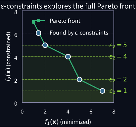
\(\varepsilon\)-Constraints: How It Works

Step-by-step process:

1. Start with the full Pareto front
2. Set an upper bound \(\varepsilon_2\) on \(f_2\)
3. Minimize \(f_1\) in the feasible region (\(f_2 \leq \varepsilon_2\))
4. Lower \(\varepsilon_2\) and repeat
5. Collected optima trace the Pareto front

Each \(\varepsilon\) value requires solving a full optimization problem.

Key advantage: By systematically varying \(\varepsilon_2\), we can explore the entire Pareto front — including unsupported non-convex points that weighted-sum methods cannot select.

{
  async function loadThemeConfig() {
    const paths = [
      "/config/graphics-colors.json",
      "../config/graphics-colors.json",
      "config/graphics-colors.json",
    ];
    for (const path of paths) {
      try {
        const response = await fetch(path);
        if (response.ok) {
          return await response.json();
        }
      } catch (error) {
        // Continue to the next path candidate.
      }
    }
    throw new Error("Could not load config/graphics-colors.json");
  }

  function hexToRgba(hexColor, alpha) {
    const clean = hexColor.replace("#", "").trim();
    const expanded = clean.length === 3
      ? clean.split("").map((char) => char + char).join("")
      : clean;
    const value = Number.parseInt(expanded, 16);
    if (Number.isNaN(value) || expanded.length !== 6) {
      return `rgba(255, 255, 255, ${alpha})`;
    }
    const red = (value >> 16) & 255;
    const green = (value >> 8) & 255;
    const blue = value & 255;
    return `rgba(${red}, ${green}, ${blue}, ${alpha})`;
  }

  const themeConfig = await loadThemeConfig();
  const selectedTheme = (
    window.GRAPHICS_THEME ??
    window.SLIDE_THEME ??
    themeConfig.default_theme
  );
  const theme = (
    themeConfig.themes[selectedTheme] ??
    themeConfig.themes[themeConfig.default_theme]
  );
  const fontConfig = themeConfig.font ?? {};
  const BG = theme.background;
  const PARETO = theme.primary;
  const ACCENT = theme.accent;
  const SECONDARY = theme.secondary;
  const ERROR = theme.error;
  const TEXT = theme.text_primary;
  const GRID = theme.grid;
  const STROKE = theme.white;
  const FONT = (
    fontConfig.ojs_css_stack ??
    '"Source Sans 3", "Inter", "Segoe UI", "DejaVu Sans", "Arial", sans-serif'
  );
  const BUTTON_BG = hexToRgba(STROKE, 0.12);
  const BUTTON_BORDER = hexToRgba(STROKE, 0.25);
  const width = 800, height = 700;
  const margin = { top: 50, right: 70, bottom: 110, left: 70 };
  const plotBaseW = width - margin.left - margin.right;
  const plotBaseH = height - margin.top - margin.bottom;
  const iSize = Math.min(plotBaseW, plotBaseH);
  const iW = iSize;
  const iH = iSize;
  const plotLeft = margin.left + (plotBaseW - iW) / 2;

  // Minimal non-convex teaching example: 5 Pareto points
  // Unsupported point (4,4) lies above hull segment (2,5)→(5,2).
  const paretoF1 = [1, 2, 4, 5, 7];
  const paretoF2 = [7, 5, 4, 2, 1];
  const paretoData = paretoF1.map((f1, i) => ({ f1, f2: paretoF2[i] }));

  function findOptimal(eps) {
    const feasible = paretoData.filter(d => d.f2 <= eps);
    if (feasible.length === 0) return null;
    return feasible.reduce((a, b) => a.f1 < b.f1 ? a : b);
  }

  // Stops chosen so each reveals a NEW optimal point
  const keyStops = [
    { eps: 7.0 },  // → (1, 7)
    { eps: 5.0 },  // → (2, 5)
    { eps: 4.0 },  // → (4, 4) — non-convex
    { eps: 2.0 },  // → (5, 2)
    { eps: 1.0 },  // → (7, 1)
  ];

  const x = d3.scaleLinear().domain([0, 8]).range([0, iW]);
  const y = d3.scaleLinear().domain([0, 8]).range([iH, 0]);
  const line = d3.line().x(d => x(d.f1)).y(d => y(d.f2)).curve(d3.curveMonotoneX);

  const container = d3.create("div").style("position", "relative");
  const svg = container.append("svg")
    .attr("viewBox", `0 0 ${width} ${height}`)
    .style("max-width", "100%").style("height", "auto")
    .style("background", BG).style("border-radius", "8px")
    .style("font-family", FONT);
  const g = svg.append("g").attr("transform", `translate(${plotLeft},${margin.top})`);

  // Grid
  for (let i = 1; i <= 7; i++) {
    g.append("line").attr("x1", x(i)).attr("x2", x(i)).attr("y1", 0).attr("y2", iH)
      .attr("stroke", GRID).attr("stroke-dasharray", "2,4").attr("opacity", 0.5);
    g.append("line").attr("x1", 0).attr("x2", iW).attr("y1", y(i)).attr("y2", y(i))
      .attr("stroke", GRID).attr("stroke-dasharray", "2,4").attr("opacity", 0.5);
  }

  // Axes
  g.append("g").attr("transform", `translate(0,${iH})`).call(d3.axisBottom(x).ticks(8))
    .call(g => g.selectAll("text").attr("fill", TEXT).style("font-size", "14px"))
    .call(g => g.selectAll("line,path").attr("stroke", TEXT).attr("opacity", 0.5));
  g.append("g").call(d3.axisLeft(y).ticks(8))
    .call(g => g.selectAll("text").attr("fill", TEXT).style("font-size", "14px"))
    .call(g => g.selectAll("line,path").attr("stroke", TEXT).attr("opacity", 0.5));

  g.append("text").attr("x", iW / 2).attr("y", iH + 45).attr("text-anchor", "middle")
    .attr("fill", TEXT).style("font-size", "16px").text("f\u2081(x) \u2014 minimized");
  g.append("text").attr("transform", "rotate(-90)").attr("x", -iH / 2).attr("y", -50)
    .attr("text-anchor", "middle").attr("fill", TEXT).style("font-size", "16px")
    .text("f\u2082(x) \u2014 constrained");

  // Title
  g.append("text").attr("x", iW / 2).attr("y", -20).attr("text-anchor", "middle")
    .attr("fill", TEXT).style("font-size", "18px").style("font-weight", "600")
    .text("Sweeping \u03b5\u2082 discovers Pareto-optimal points");

  // Legend (bottom row, one item per column)
  const legend = svg.append("g").attr("transform", `translate(${plotLeft + 6}, ${height - 28})`);
  const legendColW = 150;
  legend.append("line").attr("x1", 0).attr("x2", 16).attr("y1", 0).attr("y2", 0)
    .attr("stroke", PARETO).attr("stroke-width", 2.5);
  legend.append("circle").attr("cx", 8).attr("cy", 0).attr("r", 4.5)
    .attr("fill", PARETO).attr("stroke", STROKE).attr("stroke-width", 1);
  legend.append("text").attr("x", 22).attr("y", 1).attr("fill", TEXT)
    .attr("dominant-baseline", "middle").style("font-size", "11px").text("Pareto front");

  legend.append("circle").attr("cx", legendColW + 8).attr("cy", 0).attr("r", 7)
    .attr("fill", SECONDARY).attr("stroke", STROKE).attr("stroke-width", 2);
  legend.append("text").attr("x", legendColW + 22).attr("y", 1).attr("fill", TEXT)
    .attr("dominant-baseline", "middle").style("font-size", "11px").text("Found by \u03b5-constraints");

  legend.append("line")
    .attr("x1", 2 * legendColW).attr("x2", 2 * legendColW + 16)
    .attr("y1", 0).attr("y2", 0)
    .attr("stroke", ACCENT).attr("stroke-width", 2).attr("stroke-dasharray", "6,4");
  legend.append("text").attr("x", 2 * legendColW + 22).attr("y", 1).attr("fill", TEXT)
    .attr("dominant-baseline", "middle").style("font-size", "11px").text("\u03b5\u2082 bound / feasible region");

  legend.append("line")
    .attr("x1", 3 * legendColW).attr("x2", 3 * legendColW + 16)
    .attr("y1", 0).attr("y2", 0)
    .attr("stroke", STROKE).attr("stroke-width", 2.5).attr("stroke-dasharray", "10,6");
  legend.append("text").attr("x", 3 * legendColW + 22).attr("y", 1).attr("fill", TEXT)
    .attr("dominant-baseline", "middle").style("font-size", "11px").text("Weighted-sum hull limit");

  legend.append("line")
    .attr("x1", 4 * legendColW).attr("x2", 4 * legendColW + 16)
    .attr("y1", 0).attr("y2", 0)
    .attr("stroke", SECONDARY).attr("stroke-width", 2).attr("stroke-dasharray", "7,5");
  legend.append("text").attr("x", 4 * legendColW + 22).attr("y", 1).attr("fill", TEXT)
    .attr("dominant-baseline", "middle").style("font-size", "11px").text("min f\u2081 search");

  // Convex hull dashed line (shows which points weighted-sum would find)
  const hullPoints = [
    { f1: 1, f2: 7 }, { f1: 2, f2: 5 }, { f1: 5, f2: 2 }, { f1: 7, f2: 1 },
  ];
  const hullLine = d3.line().x(d => x(d.f1)).y(d => y(d.f2));
  g.append("path").datum(hullPoints).attr("d", hullLine)
    .attr("fill", "none").attr("stroke", STROKE)
    .attr("stroke-width", 2.5).attr("stroke-dasharray", "10,6").attr("opacity", 0.4);

  // Shaded gap between hull and front (non-convex region)
  g.append("path")
    .attr("d", `M${x(2)},${y(5)} L${x(5)},${y(2)} L${x(4)},${y(4)} Z`)
    .attr("fill", ACCENT).attr("opacity", 0.08);
  g.append("text").attr("x", x(4.1)).attr("y", y(3.35))
    .attr("text-anchor", "middle").attr("fill", ACCENT).style("font-size", "11px")
    .style("font-style", "italic").attr("opacity", 0.6).text("non-convex region");

  // Non-convex point index (f1=4)
  const ncIndices = new Set([4]);

  // Pareto front curve + dots
  g.append("path").datum(paretoData).attr("d", line)
    .attr("fill", "none").attr("stroke", PARETO).attr("stroke-width", 2.5);
  g.selectAll(".pareto-pt").data(paretoData).join("circle")
    .attr("cx", d => x(d.f1)).attr("cy", d => y(d.f2))
    .attr("r", 5).attr("fill", PARETO).attr("stroke", STROKE).attr("stroke-width", 1);

  // Animated elements
  const feasibleRect = g.append("rect")
    .attr("x", 0).attr("width", iW).attr("y", y(8)).attr("height", 0)
    .attr("fill", ACCENT).attr("opacity", 0);
  const epsLine2 = g.append("line")
    .attr("x1", 0).attr("x2", iW).attr("y1", y(8)).attr("y2", y(8))
    .attr("stroke", ACCENT).attr("stroke-width", 2).attr("stroke-dasharray", "8,5")
    .attr("opacity", 0);
  const epsLabel = g.append("text")
    .attr("x", iW + 5).attr("y", y(8)).attr("fill", ACCENT)
    .attr("dominant-baseline", "middle").style("font-size", "16px").style("font-weight", "600")
    .attr("opacity", 0);
  const solveCounter = g.append("text")
    .attr("x", iW).attr("y", -5).attr("text-anchor", "end")
    .attr("fill", ACCENT).style("font-size", "16px").style("font-weight", "600")
    .text("Solves: 0");
  const minLayer = g.append("g");
  const minLine = minLayer.append("line")
    .attr("stroke", SECONDARY).attr("stroke-width", 2)
    .attr("stroke-dasharray", "7,5").attr("opacity", 0);
  const minLabel = minLayer.append("text")
    .attr("fill", SECONDARY).style("font-size", "12px").style("font-weight", "600")
    .attr("opacity", 0);

  const foundGroup = g.append("g");
  const delay = ms => new Promise(r => setTimeout(r, ms));
  const fullSweepStopIndices = new Set([0, 2, 4]);

  async function animateMinSearch(eps, targetF1, mode = "short") {
    const yTop = y(eps);
    const yBottom = y(0);
    const xStart = x(8);
    const xTarget = x(targetF1);

    minLine.interrupt()
      .attr("x1", xStart).attr("x2", xStart)
      .attr("y1", yTop).attr("y2", yBottom)
      .attr("opacity", 0.95);
    minLabel.interrupt()
      .attr("x", x(0.8))
      .attr("y", Math.max(14, yTop - 8))
      .text("min f\u2081: move left")
      .attr("opacity", 0.95);

    if (mode === "full") {
      await minLine.transition().duration(420).ease(d3.easeCubicOut)
        .attr("x1", xTarget).attr("x2", xTarget).end();
      await delay(150);
    } else {
      const cueF1 = Math.min(7.8, targetF1 + 0.8);
      await minLine.transition().duration(170).ease(d3.easeCubicOut)
        .attr("x1", x(cueF1)).attr("x2", x(cueF1)).end();
      await minLine.transition().duration(120).ease(d3.easeLinear)
        .attr("x1", xTarget).attr("x2", xTarget).end();
      await delay(80);
    }

    await minLine.transition().duration(120).attr("opacity", 0).end();
    minLabel.transition().duration(120).attr("opacity", 0);
  }

  async function animate() {
    foundGroup.selectAll("*").remove();
    solveCounter.text("Solves: 0");
    minLine.interrupt().attr("opacity", 0);
    minLabel.interrupt().attr("opacity", 0).text("");
    epsLine2.attr("y1", y(8)).attr("y2", y(8)).attr("opacity", 1);
    epsLabel.attr("y", y(8)).text("\u03b5\u2082 = 8").attr("opacity", 1);
    feasibleRect.attr("y", y(8)).attr("height", y(0) - y(8)).attr("opacity", 0.08);
    await delay(500);

    let solveCount = 0, prevEps = 8;
    const alreadyFound = new Set();

    for (let stopIdx = 0; stopIdx < keyStops.length; stopIdx += 1) {
      const stop = keyStops[stopIdx];
      const dur = 800 + Math.abs(prevEps - stop.eps) * 150;

      await epsLine2.transition().duration(dur).ease(d3.easeLinear)
        .attr("y1", y(stop.eps)).attr("y2", y(stop.eps)).end();
      feasibleRect.transition().duration(dur).ease(d3.easeLinear)
        .attr("y", y(stop.eps)).attr("height", y(0) - y(stop.eps));
      epsLabel.transition().duration(dur).ease(d3.easeLinear)
        .attr("y", y(stop.eps)).tween("text", function() {
          const interp = d3.interpolateNumber(prevEps, stop.eps);
          return t => d3.select(this).text(`\u03b5\u2082 = ${interp(t).toFixed(1)}`);
        });
      await delay(dur);

      solveCount++;
      solveCounter.text(`Solves: ${solveCount}`);

      const fp = findOptimal(stop.eps);
      if (fp) {
        const sweepMode = fullSweepStopIndices.has(stopIdx) ? "full" : "short";
        await animateMinSearch(stop.eps, fp.f1, sweepMode);

        const key = `${fp.f1},${fp.f2}`;
        if (!alreadyFound.has(key)) {
          alreadyFound.add(key);
          const pt = foundGroup.append("circle")
            .attr("cx", x(fp.f1)).attr("cy", y(fp.f2))
            .attr("r", 0).attr("fill", SECONDARY)
            .attr("stroke", STROKE).attr("stroke-width", 2.5);
          await pt.transition().duration(400).ease(d3.easeBackOut).attr("r", 10).end();

          // Label: show coordinate and highlight non-convex points
          const isNC = ncIndices.has(fp.f1);
          const labelColor = isNC ? ACCENT : TEXT;
          const labelText = isNC
            ? `(${fp.f1}, ${fp.f2}) \u2190 non-convex!`
            : `min f\u2081 = ${fp.f1}`;
          foundGroup.append("text")
            .attr("x", x(fp.f1)).attr("y", y(fp.f2) - 16)
            .attr("text-anchor", "middle")
            .attr("fill", labelColor).style("font-size", isNC ? "13px" : "12px")
            .style("font-weight", isNC ? "600" : "400")
            .text(labelText)
            .attr("opacity", 0).transition().duration(300).attr("opacity", 1);

          // Extra ring highlight for non-convex points
          if (isNC) {
            foundGroup.append("circle")
              .attr("cx", x(fp.f1)).attr("cy", y(fp.f2))
              .attr("r", 10).attr("fill", "none").attr("stroke", ACCENT)
              .attr("stroke-width", 2.5).attr("opacity", 0)
              .transition().duration(400).attr("opacity", 1).attr("r", 15)
              .transition().duration(300).attr("r", 12).attr("opacity", 0.7);
          }
        }
      }
      prevEps = stop.eps;
      await delay(700);
    }
    epsLabel.text("\u03b5\u2082 = " + keyStops[keyStops.length - 1].eps);
  }

  container.append("button").text("\u25b6 Replay")
    .style("position", "absolute").style("top", "8px").style("left", "8px")
    .style("background", BUTTON_BG).style("color", TEXT)
    .style("border", `1px solid ${BUTTON_BORDER}`).style("border-radius", "4px")
    .style("padding", "4px 12px").style("cursor", "pointer")
    .style("font-family", FONT).style("font-size", "13px")
    .on("click", () => animate());

  const node = container.node();
  const obs = new IntersectionObserver((entries) => {
    if (entries[0].isIntersecting) { animate(); obs.disconnect(); }
  }, { threshold: 0.3 });
  requestAnimationFrame(() => obs.observe(node));

  yield node;
}

Figure 50

\(\varepsilon\)-Constraints: Infeasible Bounds

Drawback 1: Infeasible bounds

If \(\varepsilon_2\) is set too tight, no Pareto point satisfies the constraint — the subproblem becomes infeasible.

The user must know the range of each objective to choose meaningful \(\varepsilon\) values.

Setting \(\varepsilon_2 < \min_{x \in \text{Pareto}} f_2(x)\) guarantees infeasibility.

{
  async function loadThemeConfig() {
    const paths = [
      "/config/graphics-colors.json",
      "../config/graphics-colors.json",
      "config/graphics-colors.json",
    ];
    for (const path of paths) {
      try {
        const response = await fetch(path);
        if (response.ok) {
          return await response.json();
        }
      } catch (error) {
        // Continue to the next path candidate.
      }
    }
    throw new Error("Could not load config/graphics-colors.json");
  }

  function hexToRgba(hexColor, alpha) {
    const clean = hexColor.replace("#", "").trim();
    const expanded = clean.length === 3
      ? clean.split("").map((char) => char + char).join("")
      : clean;
    const value = Number.parseInt(expanded, 16);
    if (Number.isNaN(value) || expanded.length !== 6) {
      return `rgba(255, 255, 255, ${alpha})`;
    }
    const red = (value >> 16) & 255;
    const green = (value >> 8) & 255;
    const blue = value & 255;
    return `rgba(${red}, ${green}, ${blue}, ${alpha})`;
  }

  const themeConfig = await loadThemeConfig();
  const selectedTheme = (
    window.GRAPHICS_THEME ??
    window.SLIDE_THEME ??
    themeConfig.default_theme
  );
  const theme = (
    themeConfig.themes[selectedTheme] ??
    themeConfig.themes[themeConfig.default_theme]
  );
  const fontConfig = themeConfig.font ?? {};
  const BG = theme.background;
  const PARETO = theme.primary;
  const ACCENT = theme.accent;
  const SECONDARY = theme.secondary;
  const ERROR = theme.error;
  const TEXT = theme.text_primary;
  const GRID = theme.grid;
  const STROKE = theme.white;
  const FONT = (
    fontConfig.ojs_css_stack ??
    '"Source Sans 3", "Inter", "Segoe UI", "DejaVu Sans", "Arial", sans-serif'
  );
  const BUTTON_BG = hexToRgba(STROKE, 0.12);
  const BUTTON_BORDER = hexToRgba(STROKE, 0.25);
  const width = 800, height = 700;
  const margin = { top: 50, right: 70, bottom: 110, left: 70 };
  const plotBaseW = width - margin.left - margin.right;
  const plotBaseH = height - margin.top - margin.bottom;
  const iSize = Math.min(plotBaseW, plotBaseH);
  const iW = iSize;
  const iH = iSize;
  const plotLeft = margin.left + (plotBaseW - iW) / 2;

  // Minimal non-convex teaching example
  const paretoF1 = [1, 2, 4, 5, 7];
  const paretoF2 = [7, 5, 4, 2, 1];
  const paretoData = paretoF1.map((f1, i) => ({ f1, f2: paretoF2[i] }));

  function findOptimal(eps) {
    const feasible = paretoData.filter(d => d.f2 <= eps);
    if (feasible.length === 0) return null;
    return feasible.reduce((a, b) => a.f1 < b.f1 ? a : b);
  }

  const x = d3.scaleLinear().domain([0, 8]).range([0, iW]);
  const y = d3.scaleLinear().domain([0, 8]).range([iH, 0]);
  const lineFn = d3.line().x(d => x(d.f1)).y(d => y(d.f2)).curve(d3.curveMonotoneX);

  const container = d3.create("div").style("position", "relative");
  const svg = container.append("svg")
    .attr("viewBox", `0 0 ${width} ${height}`)
    .style("max-width", "100%").style("height", "auto")
    .style("background", BG).style("border-radius", "8px")
    .style("font-family", FONT);
  const g = svg.append("g").attr("transform", `translate(${plotLeft},${margin.top})`);

  for (let i = 1; i <= 7; i++) {
    g.append("line").attr("x1", x(i)).attr("x2", x(i)).attr("y1", 0).attr("y2", iH)
      .attr("stroke", GRID).attr("stroke-dasharray", "2,4").attr("opacity", 0.5);
    g.append("line").attr("x1", 0).attr("x2", iW).attr("y1", y(i)).attr("y2", y(i))
      .attr("stroke", GRID).attr("stroke-dasharray", "2,4").attr("opacity", 0.5);
  }
  g.append("g").attr("transform", `translate(0,${iH})`).call(d3.axisBottom(x).ticks(8))
    .call(g => g.selectAll("text").attr("fill", TEXT).style("font-size", "14px"))
    .call(g => g.selectAll("line,path").attr("stroke", TEXT).attr("opacity", 0.5));
  g.append("g").call(d3.axisLeft(y).ticks(8))
    .call(g => g.selectAll("text").attr("fill", TEXT).style("font-size", "14px"))
    .call(g => g.selectAll("line,path").attr("stroke", TEXT).attr("opacity", 0.5));
  g.append("text").attr("x", iW / 2).attr("y", iH + 45).attr("text-anchor", "middle")
    .attr("fill", TEXT).style("font-size", "16px").text("f\u2081(x) \u2014 minimized");
  g.append("text").attr("transform", "rotate(-90)").attr("x", -iH / 2).attr("y", -50)
    .attr("text-anchor", "middle").attr("fill", TEXT).style("font-size", "16px")
    .text("f\u2082(x) \u2014 constrained");
  g.append("text").attr("x", iW / 2).attr("y", -20).attr("text-anchor", "middle")
    .attr("fill", TEXT).style("font-size", "18px").style("font-weight", "600")
    .text("What happens when \u03b5\u2082 is too tight?");

  // Legend (bottom row, one item per column)
  const legend = svg.append("g").attr("transform", `translate(${plotLeft + 50}, ${height - 28})`);
  const legendColW = 210;
  legend.append("line").attr("x1", 0).attr("x2", 16).attr("y1", 0).attr("y2", 0)
    .attr("stroke", PARETO).attr("stroke-width", 2.5);
  legend.append("circle").attr("cx", 8).attr("cy", 0).attr("r", 4.5)
    .attr("fill", PARETO).attr("stroke", STROKE).attr("stroke-width", 1);
  legend.append("text").attr("x", 22).attr("y", 1).attr("fill", TEXT)
    .attr("dominant-baseline", "middle").style("font-size", "11px").text("Pareto front");

  legend.append("line")
    .attr("x1", legendColW).attr("x2", legendColW + 16)
    .attr("y1", 0).attr("y2", 0)
    .attr("stroke", ACCENT).attr("stroke-width", 2).attr("stroke-dasharray", "6,4");
  legend.append("text").attr("x", legendColW + 22).attr("y", 1).attr("fill", TEXT)
    .attr("dominant-baseline", "middle").style("font-size", "11px").text("\u03b5\u2082 bound");

  legend.append("line")
    .attr("x1", 2 * legendColW).attr("x2", 2 * legendColW + 16)
    .attr("y1", 0).attr("y2", 0)
    .attr("stroke", SECONDARY).attr("stroke-width", 2).attr("stroke-dasharray", "7,5");
  legend.append("text").attr("x", 2 * legendColW + 22).attr("y", 1).attr("fill", TEXT)
    .attr("dominant-baseline", "middle").style("font-size", "11px").text("min f\u2081 search");

  g.append("path").datum(paretoData).attr("d", lineFn)
    .attr("fill", "none").attr("stroke", PARETO).attr("stroke-width", 2.5);
  g.selectAll(".pd").data(paretoData).join("circle")
    .attr("cx", d => x(d.f1)).attr("cy", d => y(d.f2))
    .attr("r", 5).attr("fill", PARETO).attr("stroke", STROKE).attr("stroke-width", 1);

  const dynamicLayer = g.append("g");
  const delay = ms => new Promise(r => setTimeout(r, ms));

  async function animate() {
    dynamicLayer.selectAll("*").remove();

    const epsLine = dynamicLayer.append("line")
      .attr("x1", 0).attr("x2", iW).attr("y1", y(8)).attr("y2", y(8))
      .attr("stroke", ACCENT).attr("stroke-width", 2).attr("stroke-dasharray", "8,5");
    const epsLabelEl = dynamicLayer.append("text")
      .attr("x", iW + 5).attr("fill", ACCENT).attr("dominant-baseline", "middle")
      .style("font-size", "16px").style("font-weight", "600").attr("y", y(8));
    const feasRect = dynamicLayer.append("rect")
      .attr("x", 0).attr("width", iW).attr("fill", ACCENT).attr("opacity", 0.08)
      .attr("y", y(8)).attr("height", 0);
    const minLayer = dynamicLayer.append("g");
    const minLine = minLayer.append("line")
      .attr("stroke", SECONDARY).attr("stroke-width", 2)
      .attr("stroke-dasharray", "7,5").attr("opacity", 0);
    const minLabel = minLayer.append("text")
      .attr("fill", SECONDARY).style("font-size", "12px").style("font-weight", "600")
      .attr("opacity", 0);

    async function animateMinSearch(eps, targetF1) {
      const yTop = y(eps);
      const yBottom = y(0);
      minLine.interrupt()
        .attr("x1", x(8)).attr("x2", x(8))
        .attr("y1", yTop).attr("y2", yBottom)
        .attr("opacity", 0.95);
      minLabel.interrupt()
        .attr("x", x(0.8))
        .attr("y", Math.max(14, yTop - 8))
        .text("min f\u2081: move left")
        .attr("opacity", 0.95);

      await minLine.transition().duration(260).ease(d3.easeCubicOut)
        .attr("x1", x(targetF1)).attr("x2", x(targetF1)).end();
      await delay(70);
      minLine.transition().duration(120).attr("opacity", 0);
      minLabel.transition().duration(120).attr("opacity", 0);
    }

    const sweepSteps = [5.0, 4.0, 2.0, 1.0];
    let prev = 8;
    for (const eps of sweepSteps) {
      const dur = 520;
      epsLine.transition().duration(dur).ease(d3.easeLinear)
        .attr("y1", y(eps)).attr("y2", y(eps));
      feasRect.transition().duration(dur).ease(d3.easeLinear)
        .attr("y", y(eps)).attr("height", y(0) - y(eps));
      epsLabelEl.transition().duration(dur).ease(d3.easeLinear)
        .attr("y", y(eps)).tween("text", function() {
          const interp = d3.interpolateNumber(prev, eps);
          return t => d3.select(this).text(`\u03b5\u2082 = ${interp(t).toFixed(1)}`);
        });
      prev = eps;
      await delay(dur + 80);

      const opt = findOptimal(eps);
      if (opt) {
        await animateMinSearch(eps, opt.f1);
      }
    }

    // Continue to eps=0.8 — INFEASIBLE (min f2 on Pareto front is 1.0)
    await epsLine.transition().duration(1000).ease(d3.easeLinear)
      .attr("y1", y(0.8)).attr("y2", y(0.8)).end();
    feasRect.transition().duration(1000).ease(d3.easeLinear)
      .attr("y", y(0.8)).attr("height", y(0) - y(0.8)).attr("fill", ERROR).attr("opacity", 0.12);
    epsLabelEl.transition().duration(1000).ease(d3.easeLinear).attr("y", y(0.8));
    epsLabelEl.text("\u03b5\u2082 = 0.8").attr("fill", ERROR);
    epsLine.attr("stroke", ERROR);

    const infeasibleY = y(0.8);
    minLine.interrupt()
      .attr("x1", x(8)).attr("x2", x(8))
      .attr("y1", infeasibleY).attr("y2", y(0))
      .attr("stroke", ERROR).attr("opacity", 0.95);
    minLabel.interrupt()
      .attr("x", x(0.8))
      .attr("y", Math.max(14, infeasibleY - 8))
      .attr("fill", ERROR)
      .text("min f\u2081: no feasible point")
      .attr("opacity", 0.95);
    await minLine.transition().duration(520).ease(d3.easeCubicOut)
      .attr("x1", x(0)).attr("x2", x(0)).end();

    await delay(400);
    dynamicLayer.append("text")
      .attr("x", iW / 2).attr("y", iH / 2).attr("text-anchor", "middle")
      .attr("fill", ERROR).style("font-size", "28px").style("font-weight", "700")
      .attr("opacity", 0).text("\u274c No feasible solution!")
      .transition().duration(400).attr("opacity", 1);
  }

  container.append("button").text("\u25b6 Replay")
    .style("position", "absolute").style("top", "8px").style("left", "8px")
    .style("background", BUTTON_BG).style("color", TEXT)
    .style("border", `1px solid ${BUTTON_BORDER}`).style("border-radius", "4px")
    .style("padding", "4px 12px").style("cursor", "pointer")
    .style("font-family", FONT).style("font-size", "13px")
    .on("click", () => animate());

  const node = container.node();
  const obs = new IntersectionObserver((entries) => {
    if (entries[0].isIntersecting) { animate(); obs.disconnect(); }
  }, { threshold: 0.3 });
  requestAnimationFrame(() => obs.observe(node));
  yield node;
}

Figure 51

\(\varepsilon\)-Constraints: Sensitivity to \(\varepsilon\) Spacing

Drawback 2: Sensitivity

Coarse \(\varepsilon\) spacing misses Pareto points.

Uniform \(\varepsilon\) spacing \(\neq\) uniform coverage of the Pareto front.

The choice of \(\varepsilon\) values determines which Pareto points are found — with no guarantee of completeness.

{
  async function loadThemeConfig() {
    const paths = [
      "/config/graphics-colors.json",
      "../config/graphics-colors.json",
      "config/graphics-colors.json",
    ];
    for (const path of paths) {
      try {
        const response = await fetch(path);
        if (response.ok) {
          return await response.json();
        }
      } catch (error) {
        // Continue to the next path candidate.
      }
    }
    throw new Error("Could not load config/graphics-colors.json");
  }

  function hexToRgba(hexColor, alpha) {
    const clean = hexColor.replace("#", "").trim();
    const expanded = clean.length === 3
      ? clean.split("").map((char) => char + char).join("")
      : clean;
    const value = Number.parseInt(expanded, 16);
    if (Number.isNaN(value) || expanded.length !== 6) {
      return `rgba(255, 255, 255, ${alpha})`;
    }
    const red = (value >> 16) & 255;
    const green = (value >> 8) & 255;
    const blue = value & 255;
    return `rgba(${red}, ${green}, ${blue}, ${alpha})`;
  }

  const themeConfig = await loadThemeConfig();
  const selectedTheme = (
    window.GRAPHICS_THEME ??
    window.SLIDE_THEME ??
    themeConfig.default_theme
  );
  const theme = (
    themeConfig.themes[selectedTheme] ??
    themeConfig.themes[themeConfig.default_theme]
  );
  const fontConfig = themeConfig.font ?? {};
  const BG = theme.background;
  const PARETO = theme.primary;
  const ACCENT = theme.accent;
  const SECONDARY = theme.secondary;
  const ERROR = theme.error;
  const TEXT = theme.text_primary;
  const GRID = theme.grid;
  const STROKE = theme.white;
  const FONT = (
    fontConfig.ojs_css_stack ??
    '"Source Sans 3", "Inter", "Segoe UI", "DejaVu Sans", "Arial", sans-serif'
  );
  const BUTTON_BG = hexToRgba(STROKE, 0.12);
  const BUTTON_BORDER = hexToRgba(STROKE, 0.25);
  const width = 800, height = 700;
  const margin = { top: 50, right: 70, bottom: 110, left: 70 };
  const plotBaseW = width - margin.left - margin.right;
  const plotBaseH = height - margin.top - margin.bottom;
  const iSize = Math.min(plotBaseW, plotBaseH);
  const iW = iSize;
  const iH = iSize;
  const plotLeft = margin.left + (plotBaseW - iW) / 2;

  // Minimal non-convex teaching example
  const paretoF1 = [1, 2, 4, 5, 7];
  const paretoF2 = [7, 5, 4, 2, 1];
  const paretoData2 = paretoF1.map((f1, i) => ({ f1, f2: paretoF2[i] }));

  function findOptimal2(eps) {
    const feasible = paretoData2.filter(d => d.f2 <= eps);
    if (feasible.length === 0) return null;
    return feasible.reduce((a, b) => a.f1 < b.f1 ? a : b);
  }

  // Compute all discoverable optima for ghost comparison
  const allOptima2 = new Map();
  for (let e = 8; e >= 1; e -= 0.05) {
    const opt = findOptimal2(e);
    if (opt) allOptima2.set(`${opt.f1},${opt.f2}`, opt);
  }

  const x = d3.scaleLinear().domain([0, 8]).range([0, iW]);
  const y = d3.scaleLinear().domain([0, 8]).range([iH, 0]);
  const lineFn = d3.line().x(d => x(d.f1)).y(d => y(d.f2)).curve(d3.curveMonotoneX);

  const container = d3.create("div").style("position", "relative");
  const svg = container.append("svg")
    .attr("viewBox", `0 0 ${width} ${height}`)
    .style("max-width", "100%").style("height", "auto")
    .style("background", BG).style("border-radius", "8px")
    .style("font-family", FONT);
  const g = svg.append("g").attr("transform", `translate(${plotLeft},${margin.top})`);

  for (let i = 1; i <= 7; i++) {
    g.append("line").attr("x1", x(i)).attr("x2", x(i)).attr("y1", 0).attr("y2", iH)
      .attr("stroke", GRID).attr("stroke-dasharray", "2,4").attr("opacity", 0.5);
    g.append("line").attr("x1", 0).attr("x2", iW).attr("y1", y(i)).attr("y2", y(i))
      .attr("stroke", GRID).attr("stroke-dasharray", "2,4").attr("opacity", 0.5);
  }
  g.append("g").attr("transform", `translate(0,${iH})`).call(d3.axisBottom(x).ticks(8))
    .call(g => g.selectAll("text").attr("fill", TEXT).style("font-size", "14px"))
    .call(g => g.selectAll("line,path").attr("stroke", TEXT).attr("opacity", 0.5));
  g.append("g").call(d3.axisLeft(y).ticks(8))
    .call(g => g.selectAll("text").attr("fill", TEXT).style("font-size", "14px"))
    .call(g => g.selectAll("line,path").attr("stroke", TEXT).attr("opacity", 0.5));
  g.append("text").attr("x", iW / 2).attr("y", iH + 45).attr("text-anchor", "middle")
    .attr("fill", TEXT).style("font-size", "16px").text("f\u2081(x) \u2014 minimized");
  g.append("text").attr("transform", "rotate(-90)").attr("x", -iH / 2).attr("y", -50)
    .attr("text-anchor", "middle").attr("fill", TEXT).style("font-size", "16px")
    .text("f\u2082(x) \u2014 constrained");

  const sceneTitle = g.append("text").attr("x", iW / 2).attr("y", -26)
    .attr("text-anchor", "middle").attr("fill", TEXT)
    .style("font-size", "18px").style("font-weight", "600");

  // Legend (bottom row, one item per column)
  const legend = svg.append("g").attr("transform", `translate(${plotLeft + 8}, ${height - 28})`);
  const legendColW = 170;
  legend.append("line").attr("x1", 0).attr("x2", 16).attr("y1", 0).attr("y2", 0)
    .attr("stroke", PARETO).attr("stroke-width", 2.5);
  legend.append("circle").attr("cx", 8).attr("cy", 0).attr("r", 4.5)
    .attr("fill", PARETO).attr("stroke", STROKE).attr("stroke-width", 1);
  legend.append("text").attr("x", 22).attr("y", 1).attr("fill", TEXT)
    .attr("dominant-baseline", "middle").style("font-size", "11px").text("Pareto front");

  legend.append("circle").attr("cx", legendColW + 8).attr("cy", 0).attr("r", 7)
    .attr("fill", SECONDARY).attr("stroke", STROKE).attr("stroke-width", 2);
  legend.append("text").attr("x", legendColW + 22).attr("y", 1).attr("fill", TEXT)
    .attr("dominant-baseline", "middle").style("font-size", "11px").text("Found by \u03b5-constraints");

  legend.append("circle").attr("cx", 2 * legendColW + 8).attr("cy", 0).attr("r", 6.5)
    .attr("fill", "none").attr("stroke", PARETO).attr("stroke-width", 2)
    .attr("stroke-dasharray", "3,3");
  legend.append("text").attr("x", 2 * legendColW + 22).attr("y", 1).attr("fill", TEXT)
    .attr("dominant-baseline", "middle").style("font-size", "11px").text("Missed Pareto points");

  legend.append("line")
    .attr("x1", 3 * legendColW).attr("x2", 3 * legendColW + 16)
    .attr("y1", 0).attr("y2", 0)
    .attr("stroke", SECONDARY).attr("stroke-width", 2).attr("stroke-dasharray", "7,5");
  legend.append("text").attr("x", 3 * legendColW + 22).attr("y", 1).attr("fill", TEXT)
    .attr("dominant-baseline", "middle").style("font-size", "11px").text("min f\u2081 search");

  g.append("path").datum(paretoData2).attr("d", lineFn)
    .attr("fill", "none").attr("stroke", PARETO).attr("stroke-width", 2.5);
  g.selectAll(".pd2").data(paretoData2).join("circle")
    .attr("cx", d => x(d.f1)).attr("cy", d => y(d.f2))
    .attr("r", 5).attr("fill", PARETO).attr("stroke", STROKE).attr("stroke-width", 1);

  const dynamicLayer = g.append("g");
  const delay = ms => new Promise(r => setTimeout(r, ms));

  async function runSweep2(epsValues, passLabel, speed) {
    dynamicLayer.selectAll("*").remove();
    const dur = speed;

    dynamicLayer.append("text")
      .attr("x", 10).attr("y", 6).attr("fill", TEXT)
      .style("font-size", "15px").style("font-weight", "600").text(passLabel);
    const counter = dynamicLayer.append("text")
      .attr("x", iW).attr("y", 24).attr("text-anchor", "end")
      .attr("fill", ACCENT).style("font-size", "16px").style("font-weight", "600")
      .text("Solves: 0  |  Found: 0");

    const epsLine = dynamicLayer.append("line")
      .attr("x1", 0).attr("x2", iW).attr("y1", y(8)).attr("y2", y(8))
      .attr("stroke", ACCENT).attr("stroke-width", 2).attr("stroke-dasharray", "8,5");
    const feasRect = dynamicLayer.append("rect")
      .attr("x", 0).attr("width", iW).attr("fill", ACCENT).attr("opacity", 0.08)
      .attr("y", y(8)).attr("height", 0);
    const epsLabelEl = dynamicLayer.append("text")
      .attr("x", iW + 5).attr("fill", ACCENT).attr("dominant-baseline", "middle")
      .style("font-size", "14px").style("font-weight", "600").attr("y", y(8));
    const minLayer = dynamicLayer.append("g");
    const minLine = minLayer.append("line")
      .attr("stroke", SECONDARY).attr("stroke-width", 2)
      .attr("stroke-dasharray", "7,5").attr("opacity", 0);
    const minLabel = minLayer.append("text")
      .attr("fill", SECONDARY).style("font-size", "12px").style("font-weight", "600")
      .attr("opacity", 0);

    async function animateMinSearch(eps, targetF1) {
      const yTop = y(eps);
      const yBottom = y(0);
      minLine.interrupt()
        .attr("x1", x(8)).attr("x2", x(8))
        .attr("y1", yTop).attr("y2", yBottom)
        .attr("opacity", 0.95);
      minLabel.interrupt()
        .attr("x", x(0.8))
        .attr("y", Math.max(14, yTop - 8))
        .text("min f\u2081: move left")
        .attr("opacity", 0.95);

      const sweepDur = Math.max(120, dur * 0.45);
      await minLine.transition().duration(sweepDur).ease(d3.easeCubicOut)
        .attr("x1", x(targetF1)).attr("x2", x(targetF1)).end();
      await delay(Math.max(40, dur * 0.1));
      minLine.transition().duration(100).attr("opacity", 0);
      minLabel.transition().duration(100).attr("opacity", 0);
    }

    let solves = 0;
    const found = new Map();

    for (const eps of epsValues) {
      await epsLine.transition().duration(dur).ease(d3.easeLinear)
        .attr("y1", y(eps)).attr("y2", y(eps)).end();
      feasRect.transition().duration(dur).ease(d3.easeLinear)
        .attr("y", y(eps)).attr("height", y(0) - y(eps));
      epsLabelEl.attr("y", y(eps)).text(`\u03b5\u2082 = ${eps}`);

      const opt = findOptimal2(eps);
      if (opt) {
        await animateMinSearch(eps, opt.f1);
      }

      solves++;
      if (opt) {
        const key = `${opt.f1},${opt.f2}`;
        if (!found.has(key)) {
          found.set(key, opt);
          const pt = dynamicLayer.append("circle")
            .attr("cx", x(opt.f1)).attr("cy", y(opt.f2))
            .attr("r", 0).attr("fill", SECONDARY).attr("stroke", STROKE).attr("stroke-width", 2);
          await pt.transition().duration(200).ease(d3.easeBackOut).attr("r", 9).end();
        }
      }
      counter.text(`Solves: ${solves}  |  Found: ${found.size}`);
      await delay(dur * 0.2);
    }

    // Show missed points as ghosts
    const missed = [...allOptima2.values()].filter(p => !found.has(`${p.f1},${p.f2}`));
    for (const mp of missed) {
      dynamicLayer.append("circle")
        .attr("cx", x(mp.f1)).attr("cy", y(mp.f2))
        .attr("r", 7).attr("fill", "none").attr("stroke", PARETO)
        .attr("stroke-width", 2).attr("stroke-dasharray", "3,3")
        .attr("opacity", 0).transition().duration(300).attr("opacity", 0.5);
    }
    dynamicLayer.append("text")
      .attr("x", iW / 2).attr("y", iH - 8).attr("text-anchor", "middle")
      .attr("fill", PARETO).style("font-size", "14px").style("font-style", "italic")
      .text(`${solves} solves \u2192 ${found.size} unique points (${missed.length} missed)`)
      .attr("opacity", 0).transition().duration(300).attr("opacity", 0.8);

    return { solves, unique: found.size, missed: missed.length };
  }

  async function animate() {
    // Pass 1: coarse
    sceneTitle.text("Coarse spacing: \u03b5 = {5.0, 1.0}");
    await runSweep2([5.0, 1.0], "Coarse: \u03b5 \u2208 {5.0, 1.0}", 700);
    await delay(2500);
    await dynamicLayer.transition().duration(400).style("opacity", 0).end();
    dynamicLayer.style("opacity", 1);

    // Pass 2: medium
    sceneTitle.text("Medium spacing: \u03b5 = {5.0, 4.0, 2.0, 1.0}");
    await runSweep2([5.0, 4.0, 2.0, 1.0], "Medium: \u03b5 \u2208 {5.0, 4.0, 2.0, 1.0}", 500);
    await delay(2500);
    await dynamicLayer.transition().duration(400).style("opacity", 0).end();
    dynamicLayer.style("opacity", 1);

    // Pass 3: fine
    sceneTitle.text("Fine spacing: \u03b5 = {8, 7.5, 7, ..., 1.0}");
    const epsFine = [];
    for (let e = 8; e >= 1.0; e -= 0.5) epsFine.push(e);
    await runSweep2(epsFine, "Fine: \u03b5 \u2208 {8, 7.5, 7, ..., 1.0}", 300);
    await delay(3000);
  }

  container.append("button").text("\u25b6 Replay")
    .style("position", "absolute").style("top", "8px").style("left", "8px")
    .style("background", BUTTON_BG).style("color", TEXT)
    .style("border", `1px solid ${BUTTON_BORDER}`).style("border-radius", "4px")
    .style("padding", "4px 12px").style("cursor", "pointer")
    .style("font-family", FONT).style("font-size", "13px")
    .on("click", () => animate());

  const node = container.node();
  const obs = new IntersectionObserver((entries) => {
    if (entries[0].isIntersecting) { animate(); obs.disconnect(); }
  }, { threshold: 0.3 });
  requestAnimationFrame(() => obs.observe(node));
  yield node;
}

Figure 52

\(\varepsilon\)-Constraints: Computational Cost

Drawback 3: Computational cost

Each \(\varepsilon\) value requires solving a full optimization problem.

Finer \(\varepsilon\) spacing gives better coverage but at linear cost in the number of solves.

Diminishing returns: many \(\varepsilon\) values map to the same optimal point, wasting computation.

{
  async function loadThemeConfig() {
    const paths = [
      "/config/graphics-colors.json",
      "../config/graphics-colors.json",
      "config/graphics-colors.json",
    ];
    for (const path of paths) {
      try {
        const response = await fetch(path);
        if (response.ok) {
          return await response.json();
        }
      } catch (error) {
        // Continue to the next path candidate.
      }
    }
    throw new Error("Could not load config/graphics-colors.json");
  }

  function hexToRgba(hexColor, alpha) {
    const clean = hexColor.replace("#", "").trim();
    const expanded = clean.length === 3
      ? clean.split("").map((char) => char + char).join("")
      : clean;
    const value = Number.parseInt(expanded, 16);
    if (Number.isNaN(value) || expanded.length !== 6) {
      return `rgba(255, 255, 255, ${alpha})`;
    }
    const red = (value >> 16) & 255;
    const green = (value >> 8) & 255;
    const blue = value & 255;
    return `rgba(${red}, ${green}, ${blue}, ${alpha})`;
  }

  const themeConfig = await loadThemeConfig();
  const selectedTheme = (
    window.GRAPHICS_THEME ??
    window.SLIDE_THEME ??
    themeConfig.default_theme
  );
  const theme = (
    themeConfig.themes[selectedTheme] ??
    themeConfig.themes[themeConfig.default_theme]
  );
  const fontConfig = themeConfig.font ?? {};
  const BG = theme.background;
  const PARETO = theme.primary;
  const ACCENT = theme.accent;
  const SECONDARY = theme.secondary;
  const ERROR = theme.error;
  const TEXT = theme.text_primary;
  const GRID = theme.grid;
  const STROKE = theme.white;
  const FONT = (
    fontConfig.ojs_css_stack ??
    '"Source Sans 3", "Inter", "Segoe UI", "DejaVu Sans", "Arial", sans-serif'
  );
  const BUTTON_BG = hexToRgba(STROKE, 0.12);
  const BUTTON_BORDER = hexToRgba(STROKE, 0.25);
  const width = 800, height = 700;
  const margin = { top: 50, right: 70, bottom: 110, left: 70 };
  const plotBaseW = width - margin.left - margin.right;
  const plotBaseH = height - margin.top - margin.bottom;
  const iSize = Math.min(plotBaseW, plotBaseH);
  const iW = iSize;
  const iH = iSize;
  const plotLeft = margin.left + (plotBaseW - iW) / 2;

  // Minimal non-convex teaching example
  const paretoF1 = [1, 2, 4, 5, 7];
  const paretoF2 = [7, 5, 4, 2, 1];
  const paretoData3 = paretoF1.map((f1, i) => ({ f1, f2: paretoF2[i] }));

  function findOptimal3(eps) {
    const feasible = paretoData3.filter(d => d.f2 <= eps);
    if (feasible.length === 0) return null;
    return feasible.reduce((a, b) => a.f1 < b.f1 ? a : b);
  }

  const x = d3.scaleLinear().domain([0, 8]).range([0, iW]);
  const y = d3.scaleLinear().domain([0, 8]).range([iH, 0]);
  const lineFn = d3.line().x(d => x(d.f1)).y(d => y(d.f2)).curve(d3.curveMonotoneX);

  const container = d3.create("div").style("position", "relative");
  const svg = container.append("svg")
    .attr("viewBox", `0 0 ${width} ${height}`)
    .style("max-width", "100%").style("height", "auto")
    .style("background", BG).style("border-radius", "8px")
    .style("font-family", FONT);
  const g = svg.append("g").attr("transform", `translate(${plotLeft},${margin.top})`);

  for (let i = 1; i <= 7; i++) {
    g.append("line").attr("x1", x(i)).attr("x2", x(i)).attr("y1", 0).attr("y2", iH)
      .attr("stroke", GRID).attr("stroke-dasharray", "2,4").attr("opacity", 0.5);
    g.append("line").attr("x1", 0).attr("x2", iW).attr("y1", y(i)).attr("y2", y(i))
      .attr("stroke", GRID).attr("stroke-dasharray", "2,4").attr("opacity", 0.5);
  }
  g.append("g").attr("transform", `translate(0,${iH})`).call(d3.axisBottom(x).ticks(8))
    .call(g => g.selectAll("text").attr("fill", TEXT).style("font-size", "14px"))
    .call(g => g.selectAll("line,path").attr("stroke", TEXT).attr("opacity", 0.5));
  g.append("g").call(d3.axisLeft(y).ticks(8))
    .call(g => g.selectAll("text").attr("fill", TEXT).style("font-size", "14px"))
    .call(g => g.selectAll("line,path").attr("stroke", TEXT).attr("opacity", 0.5));
  g.append("text").attr("x", iW / 2).attr("y", iH + 45).attr("text-anchor", "middle")
    .attr("fill", TEXT).style("font-size", "16px").text("f\u2081(x) \u2014 minimized");
  g.append("text").attr("transform", "rotate(-90)").attr("x", -iH / 2).attr("y", -50)
    .attr("text-anchor", "middle").attr("fill", TEXT).style("font-size", "16px")
    .text("f\u2082(x) \u2014 constrained");
  g.append("text").attr("x", iW / 2).attr("y", -26).attr("text-anchor", "middle")
    .attr("fill", TEXT).style("font-size", "18px").style("font-weight", "600")
    .text("More solves \u2260 proportionally more points");

  // Legend (bottom row, one item per column)
  const legend = svg.append("g").attr("transform", `translate(${plotLeft + 50}, ${height - 28})`);
  const legendColW = 210;
  legend.append("line").attr("x1", 0).attr("x2", 16).attr("y1", 0).attr("y2", 0)
    .attr("stroke", PARETO).attr("stroke-width", 2.5);
  legend.append("circle").attr("cx", 8).attr("cy", 0).attr("r", 4.5)
    .attr("fill", PARETO).attr("stroke", STROKE).attr("stroke-width", 1);
  legend.append("text").attr("x", 22).attr("y", 1).attr("fill", TEXT)
    .attr("dominant-baseline", "middle").style("font-size", "11px").text("Pareto front");

  legend.append("circle").attr("cx", legendColW + 8).attr("cy", 0).attr("r", 7)
    .attr("fill", SECONDARY).attr("stroke", STROKE).attr("stroke-width", 2);
  legend.append("text").attr("x", legendColW + 22).attr("y", 1).attr("fill", TEXT)
    .attr("dominant-baseline", "middle").style("font-size", "11px").text("Found by \u03b5-constraints");

  legend.append("line")
    .attr("x1", 2 * legendColW).attr("x2", 2 * legendColW + 16)
    .attr("y1", 0).attr("y2", 0)
    .attr("stroke", SECONDARY).attr("stroke-width", 2).attr("stroke-dasharray", "7,5");
  legend.append("text").attr("x", 2 * legendColW + 22).attr("y", 1).attr("fill", TEXT)
    .attr("dominant-baseline", "middle").style("font-size", "11px").text("min f\u2081 search");

  g.append("path").datum(paretoData3).attr("d", lineFn)
    .attr("fill", "none").attr("stroke", PARETO).attr("stroke-width", 2.5);
  g.selectAll(".pd3").data(paretoData3).join("circle")
    .attr("cx", d => x(d.f1)).attr("cy", d => y(d.f2))
    .attr("r", 5).attr("fill", PARETO).attr("stroke", STROKE).attr("stroke-width", 1);

  const dynamicLayer = g.append("g");
  const delay = ms => new Promise(r => setTimeout(r, ms));

  async function animate() {
    dynamicLayer.selectAll("*").remove();

    // Very fine sweep: eps from 8 down to 1.0 in steps of 0.5 (15 solves)
    const epsValues = [];
    for (let e = 8; e >= 1.0; e -= 0.5) epsValues.push(e);

    const counter = dynamicLayer.append("text")
      .attr("x", iW).attr("y", 10).attr("text-anchor", "end")
      .attr("fill", ACCENT).style("font-size", "16px").style("font-weight", "600")
      .text("Solves: 0  |  New: 0  |  Duplicate: 0");

    const epsLine = dynamicLayer.append("line")
      .attr("x1", 0).attr("x2", iW).attr("y1", y(8)).attr("y2", y(8))
      .attr("stroke", ACCENT).attr("stroke-width", 2).attr("stroke-dasharray", "8,5");
    const feasRect = dynamicLayer.append("rect")
      .attr("x", 0).attr("width", iW).attr("fill", ACCENT).attr("opacity", 0.08)
      .attr("y", y(8)).attr("height", 0);
    const epsLabelEl = dynamicLayer.append("text")
      .attr("x", iW + 5).attr("fill", ACCENT).attr("dominant-baseline", "middle")
      .style("font-size", "14px").style("font-weight", "600").attr("y", y(8));
    const minLayer = dynamicLayer.append("g");
    const minLine = minLayer.append("line")
      .attr("stroke", SECONDARY).attr("stroke-width", 2)
      .attr("stroke-dasharray", "7,5").attr("opacity", 0);
    const minLabel = minLayer.append("text")
      .attr("fill", SECONDARY).style("font-size", "12px").style("font-weight", "600")
      .attr("opacity", 0);

    async function animateMinSearch(eps, targetF1, sweepDur) {
      const yTop = y(eps);
      const yBottom = y(0);
      minLine.interrupt()
        .attr("x1", x(8)).attr("x2", x(8))
        .attr("y1", yTop).attr("y2", yBottom)
        .attr("opacity", 0.95);
      minLabel.interrupt()
        .attr("x", x(0.8))
        .attr("y", Math.max(14, yTop - 8))
        .text("min f\u2081: move left")
        .attr("opacity", 0.95);

      const moveDur = Math.max(100, sweepDur * 0.55);
      await minLine.transition().duration(moveDur).ease(d3.easeCubicOut)
        .attr("x1", x(targetF1)).attr("x2", x(targetF1)).end();
      await delay(40);
      minLine.transition().duration(90).attr("opacity", 0);
      minLabel.transition().duration(90).attr("opacity", 0);
    }

    let solves = 0, newFound = 0, duplicates = 0;
    const found = new Set();

    for (const eps of epsValues) {
      const dur = 200;
      await epsLine.transition().duration(dur).ease(d3.easeLinear)
        .attr("y1", y(eps)).attr("y2", y(eps)).end();
      feasRect.transition().duration(dur).ease(d3.easeLinear)
        .attr("y", y(eps)).attr("height", y(0) - y(eps));
      epsLabelEl.attr("y", y(eps)).text(`\u03b5\u2082 = ${eps}`);

      solves++;
      const opt = findOptimal3(eps);
      if (opt) {
        await animateMinSearch(eps, opt.f1, dur);
        const key = `${opt.f1},${opt.f2}`;
        if (!found.has(key)) {
          found.add(key);
          newFound++;
          dynamicLayer.append("circle")
            .attr("cx", x(opt.f1)).attr("cy", y(opt.f2))
            .attr("r", 0).attr("fill", SECONDARY).attr("stroke", STROKE).attr("stroke-width", 2)
            .transition().duration(200).ease(d3.easeBackOut).attr("r", 9);
        } else {
          duplicates++;
          // Flash the existing point to show it was a duplicate solve
          dynamicLayer.append("circle")
            .attr("cx", x(opt.f1)).attr("cy", y(opt.f2))
            .attr("r", 14).attr("fill", "none").attr("stroke", ERROR)
            .attr("stroke-width", 2).attr("opacity", 0.8)
            .transition().duration(400).attr("r", 20).attr("opacity", 0).remove();
        }
      } else {
        duplicates++;
      }
      counter.text(`Solves: ${solves}  |  New: ${newFound}  |  Wasted: ${duplicates}`);
      await delay(dur * 0.3);
    }

    // Final summary
    await delay(500);
    dynamicLayer.append("text")
      .attr("x", iW / 2).attr("y", iH - 8).attr("text-anchor", "middle")
      .attr("fill", ERROR).style("font-size", "15px").style("font-weight", "600")
      .text(`${solves} optimization solves for only ${newFound} unique Pareto points!`)
      .attr("opacity", 0).transition().duration(400).attr("opacity", 0.9);
  }

  container.append("button").text("\u25b6 Replay")
    .style("position", "absolute").style("top", "8px").style("left", "8px")
    .style("background", BUTTON_BG).style("color", TEXT)
    .style("border", `1px solid ${BUTTON_BORDER}`).style("border-radius", "4px")
    .style("padding", "4px 12px").style("cursor", "pointer")
    .style("font-family", FONT).style("font-size", "13px")
    .on("click", () => animate());

  const node = container.node();
  const obs = new IntersectionObserver((entries) => {
    if (entries[0].isIntersecting) { animate(); obs.disconnect(); }
  }, { threshold: 0.3 });
  requestAnimationFrame(() => obs.observe(node));
  yield node;
}

Figure 53

Mathematical Formulation

For our discrete selection problem, we minimize one objective (e.g., distance) subject to upper bounds on the others.

Decision variables:

\[ z_s \in \{0, 1\}, \quad s \in \text{Solutions} \]

\(\varepsilon\)-constraint formulation (minimize distance):

\[ \min \sum_{s \in \text{Solutions}} f_{\text{dist}}^s \cdot z_s \]

subject to:

\[ \sum_{s \in \text{Solutions}} f_{\text{wait}}^s \cdot z_s \leq \varepsilon_{\text{wait}} \]

\[ \sum_{s \in \text{Solutions}} SR^s \cdot z_s \geq \rho_{\text{service}} \]

\[ \sum_{s \in \text{Solutions}} f_{\text{fleet}}^s \cdot z_s \leq \varepsilon_{\text{fleet}} \]

\[ \sum_{s \in \text{Solutions}} z_s = 1, \quad z_s \in \{0, 1\} \]

Miettinen’s theorem (Miettinen 1994): Every solution to this problem is a weak Pareto optimum.

Implementation and Results

Listing 12: ε-constraints method: minimize distance subject to budgets on total waiting, minimum service rate, and fleet size.

def eps_select(
    eps_wait: int,
    min_service_rate: int,
    eps_fleet: int,
) -> tuple[str | None, tuple[int, int, int, int] | None]:
    """
    Select solution minimizing distance subject to
    upper bounds (epsilon values) on other objectives.

    Args:
        eps_wait: Maximum total waiting time
        min_service_rate: Minimum acceptable service rate (% served)
        eps_fleet: Maximum fleet size

    Returns:
        (solution_id, objectives) or (None, None)
        if infeasible
    """
    # Create optimization problem
    prob = LpProblem("MO_Eps", LpMinimize)

    # Binary variables
    z = LpVariable.dicts(
        "z",
        list(solutions),
        cat="Binary"
    )

    # Objective: minimize distance
    prob += lpSum(
        solutions[sid]["f_dist"] * z[sid]
        for sid in solutions
    )

    # Constraint: select exactly one
    prob += lpSum(z[sid] for sid in solutions) == 1

    # Epsilon constraints on other objectives
    prob += lpSum(
        solutions[sid]["f_wait"] * z[sid]
        for sid in solutions
    ) <= eps_wait

    prob += lpSum(
        solutions[sid]["service_rate"] * z[sid]
        for sid in solutions
    ) >= min_service_rate

    prob += lpSum(
        solutions[sid]["f_fleet"] * z[sid]
        for sid in solutions
    ) <= eps_fleet

    # Solve
    status = prob.solve(PULP_CBC_CMD(msg=0))

    # Check feasibility
    if status != 1:
        return None, None

    # Extract solution
    selected = next(
        sid for sid in solutions
        if value(z[sid]) > 0.5
    )

    return selected, objective_tuple(selected)

Listing 13: Varying the waiting budget \(\varepsilon_{\text{wait}}\) explores different trade-offs while enforcing a minimum service rate.

# Vary waiting-time budget across observed values
wait_budgets = sorted(selectable_df["f_wait"].unique())
probe_budgets = wait_budgets[: min(5, len(wait_budgets))]

for eps_wait in probe_budgets:
    sid, vals = eps_select(
        eps_wait=eps_wait,
        min_service_rate=100,
        eps_fleet=2
    )

    if sid is None:
        print(f"ε_wait={eps_wait}: INFEASIBLE\n")
    else:
        print(f"ε_wait={eps_wait}:")
        print(f"  Solution: {sid}")
        print(f"  dist={vals[0]}, wait={vals[1]}")
        print(f"  SR={vals[2]}%, fleet={vals[3]}\n")

ε_wait=2:
  Solution: S3
  dist=4, wait=2
  SR=100%, fleet=2

ε_wait=6:
  Solution: S3
  dist=4, wait=2
  SR=100%, fleet=2

ε_wait=8:
  Solution: S3
  dist=4, wait=2
  SR=100%, fleet=2

ε_wait=10:
  Solution: S3
  dist=4, wait=2
  SR=100%, fleet=2

ε_wait=12:
  Solution: S3
  dist=4, wait=2
  SR=100%, fleet=2

Interpretation:

• Tight budgets (e.g., \(\varepsilon_{\text{wait}} = 10\)) may exclude all solutions → infeasible
• Relaxed budgets allow the solver to prioritize distance minimization
• Systematically varying \(\varepsilon\) and \(\rho_{\text{service}}\) generates the Pareto set

Goal Programming

Method 3

Target-seeking optimization with explicit deviation control

03

Before the Math: What Goal Programming Tries to Do

You pick target values and minimize how far you miss them.

{
  async function loadThemeConfigGpToc1() {
    const paths = [
      "/config/graphics-colors.json",
      "../config/graphics-colors.json",
      "config/graphics-colors.json",
    ];
    for (const path of paths) {
      try {
        const response = await fetch(path);
        if (response.ok) {
          return await response.json();
        }
      } catch (error) {
        // Try next path.
      }
    }
    throw new Error("Could not load config/graphics-colors.json");
  }

  function hexToRgbaGpToc1(hexColor, alpha) {
    const clean = hexColor.replace("#", "").trim();
    const expanded = clean.length === 3
      ? clean.split("").map((char) => char + char).join("")
      : clean;
    const value = Number.parseInt(expanded, 16);
    if (Number.isNaN(value) || expanded.length !== 6) {
      return `rgba(255, 255, 255, ${alpha})`;
    }
    return `rgba(${(value >> 16) & 255}, ${(value >> 8) & 255}, ${value & 255}, ${alpha})`;
  }

  const cfg = await loadThemeConfigGpToc1();
  const selected = window.GRAPHICS_THEME ?? window.SLIDE_THEME ?? cfg.default_theme;
  const theme = cfg.themes[selected] ?? cfg.themes[cfg.default_theme];
  const fontCfg = cfg.font ?? {};

  const BG = theme.background;
  const ACCENT = theme.accent;
  const TEXT = theme.text_primary;
  const STROKE = theme.white;
  const MUTED = hexToRgbaGpToc1(TEXT, 0.32);
  const PANEL = hexToRgbaGpToc1(STROKE, 0.08);
  const PANEL_BORDER = hexToRgbaGpToc1(STROKE, 0.26);

  const FONT = fontCfg.ojs_css_stack ??
    '"Source Sans 3", "Inter", "Segoe UI", "DejaVu Sans", "Arial", sans-serif';

  const totalW = 860;
  const totalH = 260;
  const container = d3.create("div").style("position", "relative");
  const svg = container.append("svg")
    .attr("viewBox", `0 0 ${totalW} ${totalH}`)
    .style("max-width", "100%")
    .style("height", "auto")
    .style("background", BG)
    .style("border-radius", "8px")
    .style("font-family", FONT);

  svg.append("text")
    .attr("x", totalW / 2).attr("y", 34)
    .attr("text-anchor", "middle")
    .attr("fill", TEXT)
    .style("font-size", "16px")
    .style("font-weight", "700")
    .text("Goal programming in four moves");

  const steps = [
    { title: "Targets" },
    { title: "Deviations" },
    { title: "Solve style" },
    { title: "Interpret" },
  ];

  const boxW = 168;
  const boxH = 64;
  const top = 92;
  const left = 58;
  const gap = 184;

  const defs = svg.append("defs");
  defs.append("marker")
    .attr("id", "arrow-gp-toc-1")
    .attr("viewBox", "0 0 10 10")
    .attr("refX", 9).attr("refY", 5)
    .attr("markerWidth", 7).attr("markerHeight", 7)
    .attr("orient", "auto-start-reverse")
    .append("path")
    .attr("d", "M 0 0 L 10 5 L 0 10 z")
    .attr("fill", MUTED);

  const arrows = svg.append("g");
  for (let i = 0; i < steps.length - 1; i += 1) {
    const x1 = left + i * gap + boxW + 10;
    const x2 = left + (i + 1) * gap - 10;
    const y = top + boxH / 2;
    arrows.append("line")
      .attr("x1", x1).attr("y1", y)
      .attr("x2", x2).attr("y2", y)
      .attr("stroke", MUTED)
      .attr("stroke-width", 2)
      .attr("marker-end", "url(#arrow-gp-toc-1)");
  }

  const box = svg.append("g").selectAll(".gp-toc-step").data(steps).join("g")
    .attr("class", "gp-toc-step")
    .attr("transform", (_, i) => `translate(${left + i * gap},${top})`);

  box.append("rect")
    .attr("width", boxW).attr("height", boxH)
    .attr("rx", 10)
    .attr("fill", PANEL)
    .attr("stroke", PANEL_BORDER)
    .attr("stroke-width", 1.2);

  box.append("text")
    .attr("x", boxW / 2).attr("y", boxH / 2 + 5)
    .attr("text-anchor", "middle")
    .attr("fill", MUTED)
    .style("font-size", "14px")
    .style("font-weight", "700")
    .text((d) => d.title);

  const status = svg.append("text")
    .attr("x", totalW / 2)
    .attr("y", 212)
    .attr("text-anchor", "middle")
    .attr("fill", ACCENT)
    .style("font-size", "13px")
    .style("font-weight", "700");

  const delay = (ms) => new Promise((resolve) => setTimeout(resolve, ms));
  let runId = 0;

  function setActive(index) {
    box.select("rect")
      .attr("fill", PANEL)
      .attr("stroke", PANEL_BORDER)
      .attr("stroke-width", 1.2);
    box.select("text").attr("fill", MUTED);

    const active = box.filter((_, i) => i === index);
    active.select("rect")
      .attr("fill", hexToRgbaGpToc1(ACCENT, 0.18))
      .attr("stroke", ACCENT)
      .attr("stroke-width", 2.0);
    active.select("text").attr("fill", TEXT);
  }

  async function animate() {
    runId += 1;
    const myId = runId;

    status.text("");
    setActive(-1);
    await delay(250);
    if (myId !== runId) return;

    for (let i = 0; i < steps.length; i += 1) {
      setActive(i);
      status.text(`Step ${i + 1}: ${steps[i].title}.`);
      await delay(900);
      if (myId !== runId) return;
    }
  }

  const buttonBg = hexToRgbaGpToc1(STROKE, 0.12);
  const buttonBorder = hexToRgbaGpToc1(STROKE, 0.25);
  container.append("button").text("Replay")
    .style("position", "absolute").style("top", "8px").style("left", "8px")
    .style("background", buttonBg).style("color", TEXT)
    .style("border", `1px solid ${buttonBorder}`).style("border-radius", "4px")
    .style("padding", "4px 12px").style("cursor", "pointer")
    .style("font-family", FONT).style("font-size", "13px")
    .on("click", () => animate());

  const node = container.node();
  const obs = new IntersectionObserver((entries) => {
    if (entries[0].isIntersecting) {
      animate();
      obs.disconnect();
    }
  }, { threshold: 0.3 });
  requestAnimationFrame(() => obs.observe(node));

  yield node;
}

Source excerpt (mo-opt.pdf, Sec. 2.3.3, book p. 21 / PDF page 11): (Maffioli and Sciomachen 2015)

Goal Programming dates back to Charnes et al. (1955) and Charnes and Cooper (1961). It does not pose the question of maximizing multiple objectives, but rather it attempts to find specific goal values of these objectives.

Source excerpt (Arora 2017, Sec. 18.9, printed p. 789 / PDF page 19): (Arora 2017)

With goal programming, goals bj are specified for each objective function fj(x). Then the total deviation from the goals sum dj is minimized, where dj is the deviation from the goal bj for the jth objective function.

Three Ways to State a Goal

\[ \begin{aligned} f_1(x) &\ge T_1\\ f_2(x) &= T_2\\ f_3(x) &\le T_3\\ x &\in S \end{aligned} \]

{
  async function loadThemeConfigGpToc2() {
    const paths = [
      "/config/graphics-colors.json",
      "../config/graphics-colors.json",
      "config/graphics-colors.json",
    ];
    for (const path of paths) {
      try {
        const response = await fetch(path);
        if (response.ok) {
          return await response.json();
        }
      } catch (error) {
        // Try next path.
      }
    }
    throw new Error("Could not load config/graphics-colors.json");
  }

  function hexToRgbaGpToc2(hexColor, alpha) {
    const clean = hexColor.replace("#", "").trim();
    const expanded = clean.length === 3
      ? clean.split("").map((char) => char + char).join("")
      : clean;
    const value = Number.parseInt(expanded, 16);
    if (Number.isNaN(value) || expanded.length !== 6) {
      return `rgba(255, 255, 255, ${alpha})`;
    }
    return `rgba(${(value >> 16) & 255}, ${(value >> 8) & 255}, ${value & 255}, ${alpha})`;
  }

  const cfg = await loadThemeConfigGpToc2();
  const selected = window.GRAPHICS_THEME ?? window.SLIDE_THEME ?? cfg.default_theme;
  const theme = cfg.themes[selected] ?? cfg.themes[cfg.default_theme];
  const fontCfg = cfg.font ?? {};

  const BG = theme.background;
  const ACCENT = theme.accent;
  const TEXT = theme.text_primary;
  const STROKE = theme.white;
  const MUTED = hexToRgbaGpToc2(TEXT, 0.34);
  const PANEL = hexToRgbaGpToc2(STROKE, 0.08);
  const PANEL_BORDER = hexToRgbaGpToc2(STROKE, 0.26);

  const FONT = fontCfg.ojs_css_stack ??
    '"Source Sans 3", "Inter", "Segoe UI", "DejaVu Sans", "Arial", sans-serif';

  const totalW = 860;
  const totalH = 360;
  const container = d3.create("div").style("position", "relative");
  const svg = container.append("svg")
    .attr("viewBox", `0 0 ${totalW} ${totalH}`)
    .style("max-width", "100%")
    .style("height", "auto")
    .style("background", BG)
    .style("border-radius", "8px")
    .style("font-family", FONT);

  const cards = [
    { sense: ">=", name: "At least" },
    { sense: "=", name: "Exact" },
    { sense: "<=", name: "At most" },
  ];

  const cardW = 320;
  const cardH = 86;
  const left = 270;
  const top = 70;
  const gap = 20;

  const row = svg.append("g").selectAll(".card").data(cards).join("g")
    .attr("class", "card")
    .attr("transform", (_, i) => `translate(${left},${top + i * (cardH + gap)})`);

  row.append("rect")
    .attr("width", cardW).attr("height", cardH)
    .attr("rx", 12)
    .attr("fill", PANEL)
    .attr("stroke", PANEL_BORDER)
    .attr("stroke-width", 1.2);

  row.append("text")
    .attr("x", 62).attr("y", 40)
    .attr("fill", MUTED)
    .style("font-size", "28px")
    .style("font-weight", "800")
    .text((d) => d.sense);

  row.append("text")
    .attr("x", 126).attr("y", 42)
    .attr("fill", MUTED)
    .style("font-size", "16px")
    .style("font-weight", "700")
    .text((d) => d.name);

  const footer = svg.append("text")
    .attr("x", totalW / 2)
    .attr("y", 320)
    .attr("text-anchor", "middle")
    .attr("fill", MUTED)
    .style("font-size", "13px")
    .style("font-weight", "700")
    .attr("opacity", 0)
    .text("All of them use the same decision variables x in S.");

  const delay = (ms) => new Promise((resolve) => setTimeout(resolve, ms));
  let runId = 0;

  function setActive(index) {
    row.select("rect")
      .attr("fill", PANEL)
      .attr("stroke", PANEL_BORDER)
      .attr("stroke-width", 1.2);
    row.selectAll("text").attr("fill", MUTED);

    const active = row.filter((_, i) => i === index);
    active.select("rect")
      .attr("fill", hexToRgbaGpToc2(ACCENT, 0.18))
      .attr("stroke", ACCENT)
      .attr("stroke-width", 2.0);
    active.selectAll("text").attr("fill", TEXT);
  }

  async function animate() {
    runId += 1;
    const myId = runId;

    setActive(-1);
    footer.attr("opacity", 0);
    await delay(260);
    if (myId !== runId) return;

    for (let i = 0; i < cards.length; i += 1) {
      setActive(i);
      await delay(760);
      if (myId !== runId) return;
    }
    footer.transition().duration(500).attr("opacity", 1);
  }

  const buttonBg = hexToRgbaGpToc2(STROKE, 0.12);
  const buttonBorder = hexToRgbaGpToc2(STROKE, 0.25);
  container.append("button").text("Replay")
    .style("position", "absolute").style("top", "8px").style("left", "8px")
    .style("background", buttonBg).style("color", TEXT)
    .style("border", `1px solid ${buttonBorder}`).style("border-radius", "4px")
    .style("padding", "4px 12px").style("cursor", "pointer")
    .style("font-family", FONT).style("font-size", "13px")
    .on("click", () => animate());

  const node = container.node();
  const obs = new IntersectionObserver((entries) => {
    if (entries[0].isIntersecting) {
      animate();
      obs.disconnect();
    }
  }, { threshold: 0.3 });
  requestAnimationFrame(() => obs.observe(node));

  yield node;
}

Source excerpt (mo-opt.pdf, Sec. 2.3.3, book p. 21 / PDF page 11): (Maffioli and Sciomachen 2015)

An example can be given by the following program: f1(x) ≥ v1 f2(x)= v2 f3(x) ≤ v3 x ∈ S.

At Least: Only the Shortfall Matters

• Transform: \(f_1(x) + d_1^- \ge T_1\), \(d_1^- \ge 0\)
• Interpretation: \(d_1^-\) is the shortfall below the goal.

{
  async function loadThemeConfigGpToc3() {
    const paths = [
      "/config/graphics-colors.json",
      "../config/graphics-colors.json",
      "config/graphics-colors.json",
    ];
    for (const path of paths) {
      try {
        const response = await fetch(path);
        if (response.ok) {
          return await response.json();
        }
      } catch (error) {
        // Try next path.
      }
    }
    throw new Error("Could not load config/graphics-colors.json");
  }

  function hexToRgbaGpToc3(hexColor, alpha) {
    const clean = hexColor.replace("#", "").trim();
    const expanded = clean.length === 3
      ? clean.split("").map((char) => char + char).join("")
      : clean;
    const value = Number.parseInt(expanded, 16);
    if (Number.isNaN(value) || expanded.length !== 6) {
      return `rgba(255, 255, 255, ${alpha})`;
    }
    return `rgba(${(value >> 16) & 255}, ${(value >> 8) & 255}, ${value & 255}, ${alpha})`;
  }

  const cfg = await loadThemeConfigGpToc3();
  const selected = window.GRAPHICS_THEME ?? window.SLIDE_THEME ?? cfg.default_theme;
  const theme = cfg.themes[selected] ?? cfg.themes[cfg.default_theme];
  const fontCfg = cfg.font ?? {};

  const BG = theme.background;
  const ACCENT = theme.accent;
  const TEXT = theme.text_primary;
  const STROKE = theme.white;
  const MUTED = hexToRgbaGpToc3(TEXT, 0.34);
  const GRID = hexToRgbaGpToc3(TEXT, 0.22);

  const FONT = fontCfg.ojs_css_stack ??
    '"Source Sans 3", "Inter", "Segoe UI", "DejaVu Sans", "Arial", sans-serif';

  const totalW = 860;
  const totalH = 300;
  const margin = { left: 90, right: 60, top: 90, bottom: 60 };

  const container = d3.create("div").style("position", "relative");
  const svg = container.append("svg")
    .attr("viewBox", `0 0 ${totalW} ${totalH}`)
    .style("max-width", "100%")
    .style("height", "auto")
    .style("background", BG)
    .style("border-radius", "8px")
    .style("font-family", FONT);

  const x = d3.scaleLinear().domain([0, 10]).range([margin.left, totalW - margin.right]);
  const y = totalH / 2;
  const target = 6.0;

  svg.append("line")
    .attr("x1", x(0)).attr("x2", x(10))
    .attr("y1", y).attr("y2", y)
    .attr("stroke", GRID).attr("stroke-width", 3).attr("stroke-linecap", "round");

  for (let t = 0; t <= 10; t += 2) {
    svg.append("line")
      .attr("x1", x(t)).attr("x2", x(t))
      .attr("y1", y - 10).attr("y2", y + 10)
      .attr("stroke", GRID).attr("stroke-width", 2);
    svg.append("text")
      .attr("x", x(t)).attr("y", y + 34)
      .attr("text-anchor", "middle")
      .attr("fill", MUTED)
      .style("font-size", "12px")
      .style("font-weight", "700")
      .text(`${t}`);
  }

  svg.append("line")
    .attr("x1", x(target)).attr("x2", x(target))
    .attr("y1", y - 28).attr("y2", y + 28)
    .attr("stroke", ACCENT).attr("stroke-width", 3);
  svg.append("text")
    .attr("x", x(target)).attr("y", y - 40)
    .attr("text-anchor", "middle")
    .attr("fill", ACCENT)
    .style("font-size", "13px")
    .style("font-weight", "800")
    .text("T1");

  const valueDot = svg.append("circle")
    .attr("cx", x(2)).attr("cy", y)
    .attr("r", 10)
    .attr("fill", TEXT)
    .attr("stroke", STROKE)
    .attr("stroke-width", 1.4);

  const dev = svg.append("g").attr("opacity", 0);
  dev.append("line").attr("stroke", ACCENT).attr("stroke-width", 4)
    .attr("stroke-linecap", "round");
  dev.append("line").attr("stroke", ACCENT).attr("stroke-width", 4);
  dev.append("line").attr("stroke", ACCENT).attr("stroke-width", 4);
  const devLabel = dev.append("text")
    .attr("fill", ACCENT)
    .style("font-size", "13px")
    .style("font-weight", "800")
    .attr("text-anchor", "middle")
    .text("d1-");

  function setDeviation(val) {
    const isShort = val < target - 1e-9;
    const x1 = x(val);
    const x2 = x(target);
    dev.attr("opacity", isShort ? 1 : 0);
    dev.selectAll("line").attr("opacity", isShort ? 1 : 0);
    dev.selectAll("line").filter((_, i) => i === 0)
      .attr("x1", x1).attr("x2", x2).attr("y1", y - 24).attr("y2", y - 24);
    dev.selectAll("line").filter((_, i) => i === 1)
      .attr("x1", x1).attr("x2", x1).attr("y1", y - 34).attr("y2", y - 14);
    dev.selectAll("line").filter((_, i) => i === 2)
      .attr("x1", x2).attr("x2", x2).attr("y1", y - 34).attr("y2", y - 14);
    devLabel.attr("x", (x1 + x2) / 2).attr("y", y - 44);
  }

  const status = svg.append("text")
    .attr("x", totalW / 2).attr("y", 40)
    .attr("text-anchor", "middle")
    .attr("fill", MUTED)
    .style("font-size", "13px")
    .style("font-weight", "700");

  const delay = (ms) => new Promise((resolve) => setTimeout(resolve, ms));
  let runId = 0;

  async function animate() {
    runId += 1;
    const myId = runId;

    status.text("Move f1(x) from below to above the target.");
    valueDot.interrupt().attr("cx", x(2));
    setDeviation(2);
    await delay(250);
    if (myId !== runId) return;

    valueDot.transition().duration(1600).attr("cx", x(8))
      .tween("dev", () => {
        const i = d3.interpolateNumber(2, 8);
        return (t) => setDeviation(i(t));
      });
    await delay(1800);
    if (myId !== runId) return;

    status.text("If f1(x) >= T1, the shortfall d1- is zero.");
  }

  const buttonBg = hexToRgbaGpToc3(STROKE, 0.12);
  const buttonBorder = hexToRgbaGpToc3(STROKE, 0.25);
  container.append("button").text("Replay")
    .style("position", "absolute").style("top", "8px").style("left", "8px")
    .style("background", buttonBg).style("color", TEXT)
    .style("border", `1px solid ${buttonBorder}`).style("border-radius", "4px")
    .style("padding", "4px 12px").style("cursor", "pointer")
    .style("font-family", FONT).style("font-size", "13px")
    .on("click", () => animate());

  const node = container.node();
  const obs = new IntersectionObserver((entries) => {
    if (entries[0].isIntersecting) {
      animate();
      obs.disconnect();
    }
  }, { threshold: 0.3 });
  requestAnimationFrame(() => obs.observe(node));

  yield node;
}

Source excerpt (mo-opt.pdf, Sec. 2.3.3, book p. 21 / PDF page 11): (Maffioli and Sciomachen 2015)

In particular, for each constraint of the type f1(x) ≥ v1 we introduce a variable s−1 such that the above constraint becomes f1(x)+ s−1 ≥ v1.

Exactly: Deviations on Both Sides

• Transform: \(f_2(x) + d_2^- - d_2^+ = T_2\), \(d_2^-, d_2^+ \ge 0\)
• Interpretation: below is \(d_2^-\), above is \(d_2^+\).

{
  async function loadThemeConfigGpToc4() {
    const paths = [
      "/config/graphics-colors.json",
      "../config/graphics-colors.json",
      "config/graphics-colors.json",
    ];
    for (const path of paths) {
      try {
        const response = await fetch(path);
        if (response.ok) {
          return await response.json();
        }
      } catch (error) {
        // Try next path.
      }
    }
    throw new Error("Could not load config/graphics-colors.json");
  }

  function hexToRgbaGpToc4(hexColor, alpha) {
    const clean = hexColor.replace("#", "").trim();
    const expanded = clean.length === 3
      ? clean.split("").map((char) => char + char).join("")
      : clean;
    const value = Number.parseInt(expanded, 16);
    if (Number.isNaN(value) || expanded.length !== 6) {
      return `rgba(255, 255, 255, ${alpha})`;
    }
    return `rgba(${(value >> 16) & 255}, ${(value >> 8) & 255}, ${value & 255}, ${alpha})`;
  }

  const cfg = await loadThemeConfigGpToc4();
  const selected = window.GRAPHICS_THEME ?? window.SLIDE_THEME ?? cfg.default_theme;
  const theme = cfg.themes[selected] ?? cfg.themes[cfg.default_theme];
  const fontCfg = cfg.font ?? {};

  const BG = theme.background;
  const ACCENT = theme.accent;
  const TEXT = theme.text_primary;
  const STROKE = theme.white;
  const MUTED = hexToRgbaGpToc4(TEXT, 0.34);
  const GRID = hexToRgbaGpToc4(TEXT, 0.22);

  const FONT = fontCfg.ojs_css_stack ??
    '"Source Sans 3", "Inter", "Segoe UI", "DejaVu Sans", "Arial", sans-serif';

  const totalW = 860;
  const totalH = 320;
  const margin = { left: 90, right: 60, top: 90, bottom: 60 };

  const container = d3.create("div").style("position", "relative");
  const svg = container.append("svg")
    .attr("viewBox", `0 0 ${totalW} ${totalH}`)
    .style("max-width", "100%")
    .style("height", "auto")
    .style("background", BG)
    .style("border-radius", "8px")
    .style("font-family", FONT);

  const x = d3.scaleLinear().domain([0, 10]).range([margin.left, totalW - margin.right]);
  const y = totalH / 2;
  const target = 5.0;

  svg.append("line")
    .attr("x1", x(0)).attr("x2", x(10))
    .attr("y1", y).attr("y2", y)
    .attr("stroke", GRID).attr("stroke-width", 3).attr("stroke-linecap", "round");

  for (let t = 0; t <= 10; t += 2) {
    svg.append("line")
      .attr("x1", x(t)).attr("x2", x(t))
      .attr("y1", y - 10).attr("y2", y + 10)
      .attr("stroke", GRID).attr("stroke-width", 2);
    svg.append("text")
      .attr("x", x(t)).attr("y", y + 34)
      .attr("text-anchor", "middle")
      .attr("fill", MUTED)
      .style("font-size", "12px")
      .style("font-weight", "700")
      .text(`${t}`);
  }

  svg.append("line")
    .attr("x1", x(target)).attr("x2", x(target))
    .attr("y1", y - 28).attr("y2", y + 28)
    .attr("stroke", ACCENT).attr("stroke-width", 3);
  svg.append("text")
    .attr("x", x(target)).attr("y", y - 40)
    .attr("text-anchor", "middle")
    .attr("fill", ACCENT)
    .style("font-size", "13px")
    .style("font-weight", "800")
    .text("T2");

  const valueDot = svg.append("circle")
    .attr("cx", x(3)).attr("cy", y)
    .attr("r", 10)
    .attr("fill", TEXT)
    .attr("stroke", STROKE)
    .attr("stroke-width", 1.4);

  const bracket = svg.append("g").attr("opacity", 0);
  bracket.append("line").attr("stroke", ACCENT).attr("stroke-width", 4)
    .attr("stroke-linecap", "round");
  bracket.append("line").attr("stroke", ACCENT).attr("stroke-width", 4);
  bracket.append("line").attr("stroke", ACCENT).attr("stroke-width", 4);
  const label = bracket.append("text")
    .attr("fill", ACCENT)
    .style("font-size", "13px")
    .style("font-weight", "800")
    .attr("text-anchor", "middle");

  function setDeviation(val) {
    const eps = 1e-9;
    if (Math.abs(val - target) <= eps) {
      bracket.attr("opacity", 0);
      return;
    }

    const isUnder = val < target;
    const x1 = x(isUnder ? val : target);
    const x2 = x(isUnder ? target : val);
    bracket.attr("opacity", 1);
    bracket.selectAll("line").attr("opacity", 1);
    bracket.selectAll("line").filter((_, i) => i === 0)
      .attr("x1", x1).attr("x2", x2).attr("y1", y - 24).attr("y2", y - 24);
    bracket.selectAll("line").filter((_, i) => i === 1)
      .attr("x1", x1).attr("x2", x1).attr("y1", y - 34).attr("y2", y - 14);
    bracket.selectAll("line").filter((_, i) => i === 2)
      .attr("x1", x2).attr("x2", x2).attr("y1", y - 34).attr("y2", y - 14);
    label.attr("x", (x1 + x2) / 2).attr("y", y - 44).text(isUnder ? "d2-" : "d2+");
  }

  const status = svg.append("text")
    .attr("x", totalW / 2).attr("y", 40)
    .attr("text-anchor", "middle")
    .attr("fill", MUTED)
    .style("font-size", "13px")
    .style("font-weight", "700");

  const delay = (ms) => new Promise((resolve) => setTimeout(resolve, ms));
  let runId = 0;

  async function animate() {
    runId += 1;
    const myId = runId;

    status.text("Below the target: show d2-. Above the target: show d2+.");
    valueDot.interrupt().attr("cx", x(3));
    setDeviation(3);
    await delay(260);
    if (myId !== runId) return;

    valueDot.transition().duration(900).attr("cx", x(7))
      .tween("dev", () => {
        const i = d3.interpolateNumber(3, 7);
        return (t) => setDeviation(i(t));
      });
    await delay(1100);
    if (myId !== runId) return;

    valueDot.transition().duration(900).attr("cx", x(5))
      .tween("dev", () => {
        const i = d3.interpolateNumber(7, 5);
        return (t) => setDeviation(i(t));
      });
  }

  const buttonBg = hexToRgbaGpToc4(STROKE, 0.12);
  const buttonBorder = hexToRgbaGpToc4(STROKE, 0.25);
  container.append("button").text("Replay")
    .style("position", "absolute").style("top", "8px").style("left", "8px")
    .style("background", buttonBg).style("color", TEXT)
    .style("border", `1px solid ${buttonBorder}`).style("border-radius", "4px")
    .style("padding", "4px 12px").style("cursor", "pointer")
    .style("font-family", FONT).style("font-size", "13px")
    .on("click", () => animate());

  const node = container.node();
  const obs = new IntersectionObserver((entries) => {
    if (entries[0].isIntersecting) {
      animate();
      obs.disconnect();
    }
  }, { threshold: 0.3 });
  requestAnimationFrame(() => obs.observe(node));

  yield node;
}

Source excerpt (mo-opt.pdf, Sec. 2.3.3, book p. 21 / PDF page 11): (Maffioli and Sciomachen 2015)

For each constraint of the type f2(x)= v2 we introduce a surplus two variables s+2 and s−2 such that the above constraint becomes f2(x)+ s−2 − s+2 = v2.

At Most: Only the Excess Matters

• Transform: \(f_3(x) - d_3^+ \le T_3\), \(d_3^+ \ge 0\)
• Interpretation: \(d_3^+\) is the excess above the goal.

{
  async function loadThemeConfigGpToc5() {
    const paths = [
      "/config/graphics-colors.json",
      "../config/graphics-colors.json",
      "config/graphics-colors.json",
    ];
    for (const path of paths) {
      try {
        const response = await fetch(path);
        if (response.ok) {
          return await response.json();
        }
      } catch (error) {
        // Try next path.
      }
    }
    throw new Error("Could not load config/graphics-colors.json");
  }

  function hexToRgbaGpToc5(hexColor, alpha) {
    const clean = hexColor.replace("#", "").trim();
    const expanded = clean.length === 3
      ? clean.split("").map((char) => char + char).join("")
      : clean;
    const value = Number.parseInt(expanded, 16);
    if (Number.isNaN(value) || expanded.length !== 6) {
      return `rgba(255, 255, 255, ${alpha})`;
    }
    return `rgba(${(value >> 16) & 255}, ${(value >> 8) & 255}, ${value & 255}, ${alpha})`;
  }

  const cfg = await loadThemeConfigGpToc5();
  const selected = window.GRAPHICS_THEME ?? window.SLIDE_THEME ?? cfg.default_theme;
  const theme = cfg.themes[selected] ?? cfg.themes[cfg.default_theme];
  const fontCfg = cfg.font ?? {};

  const BG = theme.background;
  const ACCENT = theme.accent;
  const TEXT = theme.text_primary;
  const STROKE = theme.white;
  const MUTED = hexToRgbaGpToc5(TEXT, 0.34);
  const GRID = hexToRgbaGpToc5(TEXT, 0.22);

  const FONT = fontCfg.ojs_css_stack ??
    '"Source Sans 3", "Inter", "Segoe UI", "DejaVu Sans", "Arial", sans-serif';

  const totalW = 860;
  const totalH = 300;
  const margin = { left: 90, right: 60, top: 90, bottom: 60 };

  const container = d3.create("div").style("position", "relative");
  const svg = container.append("svg")
    .attr("viewBox", `0 0 ${totalW} ${totalH}`)
    .style("max-width", "100%")
    .style("height", "auto")
    .style("background", BG)
    .style("border-radius", "8px")
    .style("font-family", FONT);

  const x = d3.scaleLinear().domain([0, 10]).range([margin.left, totalW - margin.right]);
  const y = totalH / 2;
  const target = 4.0;

  svg.append("line")
    .attr("x1", x(0)).attr("x2", x(10))
    .attr("y1", y).attr("y2", y)
    .attr("stroke", GRID).attr("stroke-width", 3).attr("stroke-linecap", "round");

  for (let t = 0; t <= 10; t += 2) {
    svg.append("line")
      .attr("x1", x(t)).attr("x2", x(t))
      .attr("y1", y - 10).attr("y2", y + 10)
      .attr("stroke", GRID).attr("stroke-width", 2);
    svg.append("text")
      .attr("x", x(t)).attr("y", y + 34)
      .attr("text-anchor", "middle")
      .attr("fill", MUTED)
      .style("font-size", "12px")
      .style("font-weight", "700")
      .text(`${t}`);
  }

  svg.append("line")
    .attr("x1", x(target)).attr("x2", x(target))
    .attr("y1", y - 28).attr("y2", y + 28)
    .attr("stroke", ACCENT).attr("stroke-width", 3);
  svg.append("text")
    .attr("x", x(target)).attr("y", y - 40)
    .attr("text-anchor", "middle")
    .attr("fill", ACCENT)
    .style("font-size", "13px")
    .style("font-weight", "800")
    .text("T3");

  const valueDot = svg.append("circle")
    .attr("cx", x(8)).attr("cy", y)
    .attr("r", 10)
    .attr("fill", TEXT)
    .attr("stroke", STROKE)
    .attr("stroke-width", 1.4);

  const dev = svg.append("g").attr("opacity", 0);
  dev.append("line").attr("stroke", ACCENT).attr("stroke-width", 4)
    .attr("stroke-linecap", "round");
  dev.append("line").attr("stroke", ACCENT).attr("stroke-width", 4);
  dev.append("line").attr("stroke", ACCENT).attr("stroke-width", 4);
  const devLabel = dev.append("text")
    .attr("fill", ACCENT)
    .style("font-size", "13px")
    .style("font-weight", "800")
    .attr("text-anchor", "middle")
    .text("d3+");

  function setDeviation(val) {
    const isExcess = val > target + 1e-9;
    const x1 = x(target);
    const x2 = x(val);
    dev.attr("opacity", isExcess ? 1 : 0);
    dev.selectAll("line").attr("opacity", isExcess ? 1 : 0);
    dev.selectAll("line").filter((_, i) => i === 0)
      .attr("x1", x1).attr("x2", x2).attr("y1", y - 24).attr("y2", y - 24);
    dev.selectAll("line").filter((_, i) => i === 1)
      .attr("x1", x1).attr("x2", x1).attr("y1", y - 34).attr("y2", y - 14);
    dev.selectAll("line").filter((_, i) => i === 2)
      .attr("x1", x2).attr("x2", x2).attr("y1", y - 34).attr("y2", y - 14);
    devLabel.attr("x", (x1 + x2) / 2).attr("y", y - 44);
  }

  const status = svg.append("text")
    .attr("x", totalW / 2).attr("y", 40)
    .attr("text-anchor", "middle")
    .attr("fill", MUTED)
    .style("font-size", "13px")
    .style("font-weight", "700");

  const delay = (ms) => new Promise((resolve) => setTimeout(resolve, ms));
  let runId = 0;

  async function animate() {
    runId += 1;
    const myId = runId;

    status.text("Move f3(x) from above to below the target.");
    valueDot.interrupt().attr("cx", x(8));
    setDeviation(8);
    await delay(250);
    if (myId !== runId) return;

    valueDot.transition().duration(1600).attr("cx", x(2))
      .tween("dev", () => {
        const i = d3.interpolateNumber(8, 2);
        return (t) => setDeviation(i(t));
      });
    await delay(1800);
    if (myId !== runId) return;

    status.text("If f3(x) <= T3, the excess d3+ is zero.");
  }

  const buttonBg = hexToRgbaGpToc5(STROKE, 0.12);
  const buttonBorder = hexToRgbaGpToc5(STROKE, 0.25);
  container.append("button").text("Replay")
    .style("position", "absolute").style("top", "8px").style("left", "8px")
    .style("background", buttonBg).style("color", TEXT)
    .style("border", `1px solid ${buttonBorder}`).style("border-radius", "4px")
    .style("padding", "4px 12px").style("cursor", "pointer")
    .style("font-family", FONT).style("font-size", "13px")
    .on("click", () => animate());

  const node = container.node();
  const obs = new IntersectionObserver((entries) => {
    if (entries[0].isIntersecting) {
      animate();
      obs.disconnect();
    }
  }, { threshold: 0.3 });
  requestAnimationFrame(() => obs.observe(node));

  yield node;
}

Source excerpt (mo-opt.pdf, Sec. 2.3.3, book p. 21 / PDF page 11): (Maffioli and Sciomachen 2015)

For each constraint of the type f3(x) ≤ v3 we introduce a variable s+3 such that the above constraint becomes f3(x) − s+3 ≤ v3.

One Score: Weighted Deviations

\[ \min \sum_{k \in \mathcal{K}} \left(\alpha_k^- d_k^- + \alpha_k^+ d_k^+\right) \]

(Weights encode how much each miss counts.)

{
  async function loadThemeConfigGpToc6() {
    const paths = [
      "/config/graphics-colors.json",
      "../config/graphics-colors.json",
      "config/graphics-colors.json",
    ];
    for (const path of paths) {
      try {
        const response = await fetch(path);
        if (response.ok) {
          return await response.json();
        }
      } catch (error) {
        // Try next path.
      }
    }
    throw new Error("Could not load config/graphics-colors.json");
  }

  function hexToRgbaGpToc6(hexColor, alpha) {
    const clean = hexColor.replace("#", "").trim();
    const expanded = clean.length === 3
      ? clean.split("").map((char) => char + char).join("")
      : clean;
    const value = Number.parseInt(expanded, 16);
    if (Number.isNaN(value) || expanded.length !== 6) {
      return `rgba(255, 255, 255, ${alpha})`;
    }
    return `rgba(${(value >> 16) & 255}, ${(value >> 8) & 255}, ${value & 255}, ${alpha})`;
  }

  const cfg = await loadThemeConfigGpToc6();
  const selected = window.GRAPHICS_THEME ?? window.SLIDE_THEME ?? cfg.default_theme;
  const theme = cfg.themes[selected] ?? cfg.themes[cfg.default_theme];
  const fontCfg = cfg.font ?? {};

  const BG = theme.background;
  const PRIMARY = theme.primary;
  const ACCENT = theme.accent;
  const TEXT = theme.text_primary;
  const STROKE = theme.white;
  const MUTED = hexToRgbaGpToc6(TEXT, 0.34);
  const PANEL = hexToRgbaGpToc6(STROKE, 0.08);
  const PANEL_BORDER = hexToRgbaGpToc6(STROKE, 0.26);

  const FONT = fontCfg.ojs_css_stack ??
    '"Source Sans 3", "Inter", "Segoe UI", "DejaVu Sans", "Arial", sans-serif';

  const data = [
    { id: "C1", d1: 1.0, d2: 3.0 },
    { id: "C2", d1: 2.0, d2: 1.0 },
    { id: "C3", d1: 0.5, d2: 2.0 },
  ];

  let w1 = 1.0;
  let w2 = 1.0;

  function score(d) {
    return w1 * d.d1 + w2 * d.d2;
  }

  const totalW = 860;
  const totalH = 360;
  const margin = { left: 80, right: 40, top: 70, bottom: 60 };

  const container = d3.create("div").style("position", "relative");
  const svg = container.append("svg")
    .attr("viewBox", `0 0 ${totalW} ${totalH}`)
    .style("max-width", "100%")
    .style("height", "auto")
    .style("background", BG)
    .style("border-radius", "8px")
    .style("font-family", FONT);

  const x = d3.scaleBand().domain(data.map((d) => d.id))
    .range([margin.left, totalW - margin.right]).padding(0.22);
  const y = d3.scaleLinear().domain([0, 10]).range([totalH - margin.bottom, margin.top]);

  svg.append("g")
    .attr("transform", `translate(0,${totalH - margin.bottom})`)
    .call(d3.axisBottom(x))
    .call((axis) => axis.selectAll("text").attr("fill", TEXT).style("font-size", "12px"))
    .call((axis) => axis.selectAll("line,path").attr("stroke", TEXT).attr("opacity", 0.55));

  svg.append("g")
    .attr("transform", `translate(${margin.left},0)`)
    .call(d3.axisLeft(y).ticks(5))
    .call((axis) => axis.selectAll("text").attr("fill", MUTED).style("font-size", "12px"))
    .call((axis) => axis.selectAll("line,path").attr("stroke", TEXT).attr("opacity", 0.30));

  svg.append("text")
    .attr("x", margin.left)
    .attr("y", 38)
    .attr("fill", MUTED)
    .style("font-size", "13px")
    .style("font-weight", "700")
    .text("Stacked bars show weighted parts of the total deviation.");

  const panel = svg.append("g").attr("transform", `translate(${totalW - 260},${margin.top - 6})`);
  panel.append("rect")
    .attr("width", 220).attr("height", 88).attr("rx", 10)
    .attr("fill", PANEL).attr("stroke", PANEL_BORDER).attr("stroke-width", 1.2);
  const wText = panel.append("text")
    .attr("x", 12).attr("y", 26)
    .attr("fill", TEXT)
    .style("font-size", "13px")
    .style("font-weight", "800");
  const winnerText = panel.append("text")
    .attr("x", 12).attr("y", 54)
    .attr("fill", ACCENT)
    .style("font-size", "13px")
    .style("font-weight", "800");

  const bars = svg.append("g").selectAll(".bar").data(data).join("g")
    .attr("transform", (d) => `translate(${x(d.id)},0)`);

  const rect1 = bars.append("rect")
    .attr("x", 0).attr("width", x.bandwidth())
    .attr("fill", PRIMARY)
    .attr("y", y(0)).attr("height", 0);
  const rect2 = bars.append("rect")
    .attr("x", 0).attr("width", x.bandwidth())
    .attr("fill", ACCENT)
    .attr("y", y(0)).attr("height", 0);

  const outline = bars.append("rect")
    .attr("x", -4).attr("width", x.bandwidth() + 8)
    .attr("fill", "none")
    .attr("stroke", ACCENT)
    .attr("stroke-width", 2.4)
    .attr("rx", 10)
    .attr("opacity", 0);

  function updateBars(duration) {
    const totals = data.map((d) => score(d));
    const winner = data[totals.indexOf(Math.min(...totals))].id;
    wText.text(`Weights: w1=${w1.toFixed(1)}, w2=${w2.toFixed(1)}`);
    winnerText.text(`Chosen: ${winner}`);

    rect1.transition().duration(duration)
      .attr("y", (d) => y(w1 * d.d1))
      .attr("height", (d) => y(0) - y(w1 * d.d1));
    rect2.transition().duration(duration)
      .attr("y", (d) => y(w1 * d.d1 + w2 * d.d2))
      .attr("height", (d) => y(w1 * d.d1) - y(w1 * d.d1 + w2 * d.d2));

    outline.transition().duration(duration)
      .attr("opacity", (d) => (d.id === winner ? 1 : 0));
  }

  const delay = (ms) => new Promise((resolve) => setTimeout(resolve, ms));
  let runId = 0;

  async function animate() {
    runId += 1;
    const myId = runId;

    w1 = 1.0;
    w2 = 1.0;
    rect1.interrupt();
    rect2.interrupt();
    outline.interrupt();
    updateBars(0);

    await delay(350);
    if (myId !== runId) return;

    updateBars(900);
    await delay(1100);
    if (myId !== runId) return;

    w2 = 3.0;
    updateBars(900);
  }

  const buttonBg = hexToRgbaGpToc6(STROKE, 0.12);
  const buttonBorder = hexToRgbaGpToc6(STROKE, 0.25);
  container.append("button").text("Replay")
    .style("position", "absolute").style("top", "8px").style("left", "8px")
    .style("background", buttonBg).style("color", TEXT)
    .style("border", `1px solid ${buttonBorder}`).style("border-radius", "4px")
    .style("padding", "4px 12px").style("cursor", "pointer")
    .style("font-family", FONT).style("font-size", "13px")
    .on("click", () => animate());

  const node = container.node();
  const obs = new IntersectionObserver((entries) => {
    if (entries[0].isIntersecting) {
      animate();
      obs.disconnect();
    }
  }, { threshold: 0.3 });
  requestAnimationFrame(() => obs.observe(node));

  yield node;
}

Source excerpt (mo-opt.pdf, Sec. 2.3.3, book p. 22 / PDF page 12): (Maffioli and Sciomachen 2015)

There are different ways of optimizing the slack/surplus variables. An example is given by the Archimedean goal programming, where the problem becomes that of minimizing a linear combination of the surplus and slack variables each one weighted by a positive coefficient α as follows: minαs−1 s−1 +αs+2 s+2 +αs−2 s−2 +αs+3 s+3 f1(x)+s−1 ≥v1 f2(x)+s−2 −s+2 = v2 f3(x)−s+3 ≤v3 s−1 ≥0 s+2 ≥0 s−2 ≥0 s+3 ≥0 x ∈S.

Source excerpt (Lecture09.pdf, slide 11 / PDF page 11): (Sudhoff 2007)

Weighted Sum Method Scalarize a set of objectives into a single objective by adding each objective pre-multiplied by a user-supplied weight Weight of an objective is chosen in proportion to the relative importance of the objective

When You Refuse Trade-offs: Priorities

With priorities, you do not compensate a critical miss with improvements elsewhere.

{
  async function loadThemeConfigGpToc7() {
    const paths = [
      "/config/graphics-colors.json",
      "../config/graphics-colors.json",
      "config/graphics-colors.json",
    ];
    for (const path of paths) {
      try {
        const response = await fetch(path);
        if (response.ok) {
          return await response.json();
        }
      } catch (error) {
        // Try next path.
      }
    }
    throw new Error("Could not load config/graphics-colors.json");
  }

  function hexToRgbaGpToc7(hexColor, alpha) {
    const clean = hexColor.replace("#", "").trim();
    const expanded = clean.length === 3
      ? clean.split("").map((char) => char + char).join("")
      : clean;
    const value = Number.parseInt(expanded, 16);
    if (Number.isNaN(value) || expanded.length !== 6) {
      return `rgba(255, 255, 255, ${alpha})`;
    }
    return `rgba(${(value >> 16) & 255}, ${(value >> 8) & 255}, ${value & 255}, ${alpha})`;
  }

  const cfg = await loadThemeConfigGpToc7();
  const selected = window.GRAPHICS_THEME ?? window.SLIDE_THEME ?? cfg.default_theme;
  const theme = cfg.themes[selected] ?? cfg.themes[cfg.default_theme];
  const fontCfg = cfg.font ?? {};

  const BG = theme.background;
  const ACCENT = theme.accent;
  const TEXT = theme.text_primary;
  const STROKE = theme.white;
  const MUTED = hexToRgbaGpToc7(TEXT, 0.34);
  const PANEL = hexToRgbaGpToc7(STROKE, 0.08);
  const PANEL_BORDER = hexToRgbaGpToc7(STROKE, 0.26);

  const FONT = fontCfg.ojs_css_stack ??
    '"Source Sans 3", "Inter", "Segoe UI", "DejaVu Sans", "Arial", sans-serif';

  const data = [
    { id: "C1", l1: 0, l2: 3, l3: 2 },
    { id: "C2", l1: 0, l2: 1, l3: 5 },
    { id: "C3", l1: 1, l2: 0, l3: 0 },
    { id: "C4", l1: 0, l2: 1, l3: 1 },
    { id: "C5", l1: 2, l2: 0, l3: 0 },
  ];

  const totalW = 860;
  const totalH = 360;
  const container = d3.create("div").style("position", "relative");
  const svg = container.append("svg")
    .attr("viewBox", `0 0 ${totalW} ${totalH}`)
    .style("max-width", "100%")
    .style("height", "auto")
    .style("background", BG)
    .style("border-radius", "8px")
    .style("font-family", FONT);

  const left = 140;
  const top = 86;
  const rowH = 44;

  svg.append("text")
    .attr("x", left).attr("y", 44)
    .attr("fill", MUTED)
    .style("font-size", "13px")
    .style("font-weight", "700")
    .text("Filter candidates level by level (L1 first, then L2, then L3).");

  const headers = [
    { key: "id", label: "Candidate" },
    { key: "l1", label: "L1" },
    { key: "l2", label: "L2" },
    { key: "l3", label: "L3" },
  ];
  const colX = { id: left - 60, l1: left + 160, l2: left + 250, l3: left + 340 };

  const table = svg.append("g").attr("transform", `translate(0,${top})`);
  table.append("rect")
    .attr("x", left - 90).attr("y", -40)
    .attr("width", 520).attr("height", rowH * (data.length + 1) + 26)
    .attr("rx", 12)
    .attr("fill", PANEL)
    .attr("stroke", PANEL_BORDER)
    .attr("stroke-width", 1.2);

  table.selectAll(".h").data(headers).join("text")
    .attr("x", (d) => colX[d.key]).attr("y", -12)
    .attr("fill", MUTED)
    .style("font-size", "13px")
    .style("font-weight", "800")
    .text((d) => d.label);

  const rows = table.selectAll(".r").data(data).join("g")
    .attr("transform", (_, i) => `translate(0,${i * rowH})`);

  rows.append("text")
    .attr("x", colX.id).attr("y", 22)
    .attr("fill", TEXT)
    .style("font-size", "14px")
    .style("font-weight", "800")
    .text((d) => d.id);

  ["l1", "l2", "l3"].forEach((k) => {
    rows.append("text")
      .attr("x", colX[k]).attr("y", 22)
      .attr("text-anchor", "middle")
      .attr("fill", TEXT)
      .style("font-size", "14px")
      .style("font-weight", "700")
      .text((d) => d[k]);
  });

  const highlight = table.append("rect")
    .attr("x", colX.l1 - 42).attr("y", -32)
    .attr("width", 84).attr("height", rowH * (data.length + 1))
    .attr("rx", 10)
    .attr("fill", hexToRgbaGpToc7(ACCENT, 0.12))
    .attr("stroke", ACCENT)
    .attr("stroke-width", 2.0)
    .attr("opacity", 0);

  const status = svg.append("text")
    .attr("x", totalW - 50).attr("y", 44)
    .attr("text-anchor", "end")
    .attr("fill", ACCENT)
    .style("font-size", "13px")
    .style("font-weight", "800");

  function setColumn(col) {
    const colBoxes = {
      l1: { x: colX.l1 - 42 },
      l2: { x: colX.l2 - 42 },
      l3: { x: colX.l3 - 42 },
    };
    if (!colBoxes[col]) return;
    highlight.attr("x", colBoxes[col].x).attr("opacity", 1);
  }

  function fadeBy(predicate) {
    rows.transition().duration(600)
      .attr("opacity", (d) => (predicate(d) ? 1 : 0.18));
  }

  const delay = (ms) => new Promise((resolve) => setTimeout(resolve, ms));
  let runId = 0;

  async function animate() {
    runId += 1;
    const myId = runId;

    highlight.attr("opacity", 0);
    rows.interrupt().attr("opacity", 1);
    status.text("");
    await delay(260);
    if (myId !== runId) return;

    status.text("Level 1");
    setColumn("l1");
    const best1 = d3.min(data, (d) => d.l1);
    fadeBy((d) => d.l1 === best1);
    await delay(1100);
    if (myId !== runId) return;

    status.text("Level 2");
    setColumn("l2");
    const survivors1 = data.filter((d) => d.l1 === best1);
    const best2 = d3.min(survivors1, (d) => d.l2);
    fadeBy((d) => d.l1 === best1 && d.l2 === best2);
    await delay(1100);
    if (myId !== runId) return;

    status.text("Level 3");
    setColumn("l3");
    const survivors2 = data.filter((d) => d.l1 === best1 && d.l2 === best2);
    const best3 = d3.min(survivors2, (d) => d.l3);
    fadeBy((d) => d.l1 === best1 && d.l2 === best2 && d.l3 === best3);
  }

  const buttonBg = hexToRgbaGpToc7(STROKE, 0.12);
  const buttonBorder = hexToRgbaGpToc7(STROKE, 0.25);
  container.append("button").text("Replay")
    .style("position", "absolute").style("top", "8px").style("left", "8px")
    .style("background", buttonBg).style("color", TEXT)
    .style("border", `1px solid ${buttonBorder}`).style("border-radius", "4px")
    .style("padding", "4px 12px").style("cursor", "pointer")
    .style("font-family", FONT).style("font-size", "13px")
    .on("click", () => animate());

  const node = container.node();
  const obs = new IntersectionObserver((entries) => {
    if (entries[0].isIntersecting) {
      animate();
      obs.disconnect();
    }
  }, { threshold: 0.3 });
  requestAnimationFrame(() => obs.observe(node));

  yield node;
}

Source excerpt (mo-opt.pdf, Sec. 2.3.3, book p. 22 / PDF page 12): (Maffioli and Sciomachen 2015)

Besides Archimedean goal programming, other approaches are the lexicographical goal programming, the interactive goal programming, the reference goal programming and the multi-criteria goal programming (see, e.g., T’kindt and Billaut, 2005).

Source excerpt (mo-opt.pdf, Sec. 2.3.4, book p. 23 / PDF page 13): (Maffioli and Sciomachen 2015)

Multi-level programming orders the n objectives according to a hierarchy. Firstly, the minimizers of the first objective function are found; secondly, the minimizers of the second most important objective are searched for, and so forth until all the objective function have been optimized on successively smaller sets.

Multi-level programming is a useful approach if the hierarchical order among the objectives is meaningful and the user is not interested in the continuous trade-off among the functions. One drawback is that optimization problems that are solved near the end of the hierarchy can be largely constrained and could become infeasible, meaning that the less important objective functions tend to have no influence on the overall optimal solution.

Source excerpt (Arora 2017, Sec. 18.7, printed p. 788 / PDF page 18): (Arora 2017)

With the lexicographic method, preferences are imposed by ordering the objective functions according to their importance or significance, rather than by assigning weights.

After You Meet the Goals: Keep Optimizing

• Use goals as bounds: \(l_i \le f_i(x) \le \varepsilon_i\)
• Then optimize inside the bounds (e.g., weighted sum): \(\min \sum_j w_j f_j(x)\)

{
  async function loadThemeConfigGpToc8() {
    const paths = [
      "/config/graphics-colors.json",
      "../config/graphics-colors.json",
      "config/graphics-colors.json",
    ];
    for (const path of paths) {
      try {
        const response = await fetch(path);
        if (response.ok) {
          return await response.json();
        }
      } catch (error) {
        // Try next path.
      }
    }
    throw new Error("Could not load config/graphics-colors.json");
  }

  function hexToRgbaGpToc8(hexColor, alpha) {
    const clean = hexColor.replace("#", "").trim();
    const expanded = clean.length === 3
      ? clean.split("").map((char) => char + char).join("")
      : clean;
    const value = Number.parseInt(expanded, 16);
    if (Number.isNaN(value) || expanded.length !== 6) {
      return `rgba(255, 255, 255, ${alpha})`;
    }
    return `rgba(${(value >> 16) & 255}, ${(value >> 8) & 255}, ${value & 255}, ${alpha})`;
  }

  const cfg = await loadThemeConfigGpToc8();
  const selected = window.GRAPHICS_THEME ?? window.SLIDE_THEME ?? cfg.default_theme;
  const theme = cfg.themes[selected] ?? cfg.themes[cfg.default_theme];
  const fontCfg = cfg.font ?? {};

  const BG = theme.background;
  const PRIMARY = theme.primary;
  const ACCENT = theme.accent;
  const TEXT = theme.text_primary;
  const GRID = theme.grid;
  const STROKE = theme.white;
  const MUTED = hexToRgbaGpToc8(TEXT, 0.30);

  const FONT = fontCfg.ojs_css_stack ??
    '"Source Sans 3", "Inter", "Segoe UI", "DejaVu Sans", "Arial", sans-serif';

  const totalW = 860;
  const totalH = 420;
  const margin = { left: 70, right: 40, top: 70, bottom: 70 };
  const plotW = totalW - margin.left - margin.right;
  const plotH = totalH - margin.top - margin.bottom;

  const container = d3.create("div").style("position", "relative");
  const svg = container.append("svg")
    .attr("viewBox", `0 0 ${totalW} ${totalH}`)
    .style("max-width", "100%")
    .style("height", "auto")
    .style("background", BG)
    .style("border-radius", "8px")
    .style("font-family", FONT);

  const g = svg.append("g").attr("transform", `translate(${margin.left},${margin.top})`);
  const x = d3.scaleLinear().domain([0, 10]).range([0, plotW]);
  const y = d3.scaleLinear().domain([0, 10]).range([plotH, 0]);

  for (let t = 0; t <= 10; t += 2) {
    g.append("line")
      .attr("x1", x(t)).attr("x2", x(t)).attr("y1", 0).attr("y2", plotH)
      .attr("stroke", GRID).attr("stroke-dasharray", "2,5").attr("opacity", 0.45);
    g.append("line")
      .attr("x1", 0).attr("x2", plotW).attr("y1", y(t)).attr("y2", y(t))
      .attr("stroke", GRID).attr("stroke-dasharray", "2,5").attr("opacity", 0.45);
  }

  g.append("g").attr("transform", `translate(0,${plotH})`).call(d3.axisBottom(x).ticks(6))
    .call((axis) => axis.selectAll("text").attr("fill", TEXT).style("font-size", "12px"))
    .call((axis) => axis.selectAll("line,path").attr("stroke", TEXT).attr("opacity", 0.55));
  g.append("g").call(d3.axisLeft(y).ticks(6))
    .call((axis) => axis.selectAll("text").attr("fill", TEXT).style("font-size", "12px"))
    .call((axis) => axis.selectAll("line,path").attr("stroke", TEXT).attr("opacity", 0.55));

  g.append("text").attr("x", plotW / 2).attr("y", plotH + 52)
    .attr("text-anchor", "middle").attr("fill", TEXT)
    .style("font-size", "14px").style("font-weight", "700")
    .text("f1(x)");
  g.append("text").attr("transform", "rotate(-90)")
    .attr("x", -plotH / 2).attr("y", -46)
    .attr("text-anchor", "middle").attr("fill", TEXT)
    .style("font-size", "14px").style("font-weight", "700")
    .text("f2(x)");

  const points = [
    { id: "A", f1: 1.2, f2: 8.8 },
    { id: "B", f1: 2.3, f2: 6.1 },
    { id: "C", f1: 3.6, f2: 4.0 },
    { id: "D", f1: 4.7, f2: 5.4 },
    { id: "E", f1: 6.0, f2: 3.2 },
    { id: "F", f1: 7.5, f2: 2.4 },
    { id: "G", f1: 8.6, f2: 4.9 },
    { id: "H", f1: 5.1, f2: 1.6 },
    { id: "I", f1: 2.1, f2: 2.6 },
    { id: "J", f1: 7.0, f2: 6.8 },
    { id: "K", f1: 4.1, f2: 7.4 },
  ];

  const bounds = { l1: 2.0, u1: 8.0, l2: 1.0, u2: 6.0 };
  const w1 = 1.0;
  const w2 = 0.6;

  function feasible(p) {
    return p.f1 >= bounds.l1 && p.f1 <= bounds.u1 && p.f2 >= bounds.l2 && p.f2 <= bounds.u2;
  }
  function cost(p) {
    return w1 * p.f1 + w2 * p.f2;
  }

  const dots = g.selectAll(".pt").data(points).join("circle")
    .attr("class", "pt")
    .attr("cx", (d) => x(d.f1)).attr("cy", (d) => y(d.f2))
    .attr("r", 6)
    .attr("fill", PRIMARY)
    .attr("stroke", STROKE)
    .attr("stroke-width", 1.2)
    .attr("opacity", 1);

  const box = g.append("rect")
    .attr("x", x(bounds.l1))
    .attr("y", y(bounds.u2))
    .attr("width", x(bounds.u1) - x(bounds.l1))
    .attr("height", y(bounds.l2) - y(bounds.u2))
    .attr("fill", hexToRgbaGpToc8(ACCENT, 0.10))
    .attr("stroke", ACCENT)
    .attr("stroke-width", 2.2)
    .attr("rx", 10)
    .attr("opacity", 0);

  const iso = g.append("line")
    .attr("stroke", ACCENT)
    .attr("stroke-width", 2.4)
    .attr("stroke-dasharray", "10,7")
    .attr("opacity", 0);

  const winnerRing = g.append("circle")
    .attr("r", 12)
    .attr("fill", "none")
    .attr("stroke", ACCENT)
    .attr("stroke-width", 3.0)
    .attr("opacity", 0);

  const status = svg.append("text")
    .attr("x", totalW / 2).attr("y", 40)
    .attr("text-anchor", "middle")
    .attr("fill", MUTED)
    .style("font-size", "13px")
    .style("font-weight", "700");

  function setIsoLine(c) {
    const f1a = 0;
    const f1b = 10;
    const f2a = (c - w1 * f1a) / w2;
    const f2b = (c - w1 * f1b) / w2;
    iso.attr("x1", x(f1a)).attr("y1", y(f2a))
      .attr("x2", x(f1b)).attr("y2", y(f2b));
  }

  const delay = (ms) => new Promise((resolve) => setTimeout(resolve, ms));
  let runId = 0;

  async function animate() {
    runId += 1;
    const myId = runId;

    status.text("Start with all candidates.");
    dots.attr("opacity", 1);
    box.attr("opacity", 0);
    iso.attr("opacity", 0);
    winnerRing.attr("opacity", 0);
    await delay(600);
    if (myId !== runId) return;

    status.text("Keep only points that satisfy the goal bounds.");
    box.transition().duration(500).attr("opacity", 1);
    dots.transition().duration(700)
      .attr("opacity", (d) => (feasible(d) ? 1 : 0.18));
    await delay(950);
    if (myId !== runId) return;

    const feas = points.filter(feasible);
    const winner = feas.reduce((a, b) => (cost(a) <= cost(b) ? a : b));
    const cMax = d3.max(feas, cost);
    const cMin = cost(winner);

    status.text("Now optimize within the feasible set (weighted sum).");
    iso.attr("opacity", 1);
    setIsoLine(cMax + 1.0);
    iso.transition().duration(1400)
      .tween("move", () => {
        const i = d3.interpolateNumber(cMax + 1.0, cMin);
        return (t) => setIsoLine(i(t));
      });
    await delay(1550);
    if (myId !== runId) return;

    winnerRing
      .attr("cx", x(winner.f1))
      .attr("cy", y(winner.f2))
      .attr("opacity", 1);
  }

  const buttonBg = hexToRgbaGpToc8(STROKE, 0.12);
  const buttonBorder = hexToRgbaGpToc8(STROKE, 0.25);
  container.append("button").text("Replay")
    .style("position", "absolute").style("top", "8px").style("left", "8px")
    .style("background", buttonBg).style("color", TEXT)
    .style("border", `1px solid ${buttonBorder}`).style("border-radius", "4px")
    .style("padding", "4px 12px").style("cursor", "pointer")
    .style("font-family", FONT).style("font-size", "13px")
    .on("click", () => animate());

  const node = container.node();
  const obs = new IntersectionObserver((entries) => {
    if (entries[0].isIntersecting) {
      animate();
      obs.disconnect();
    }
  }, { threshold: 0.3 });
  requestAnimationFrame(() => obs.observe(node));

  yield node;
}

Source excerpt (Arora 2017, Sec. 18.8, printed p. 788 / PDF page 18): (Arora 2017)

The bounded objective function method minimizes the single most important objective function fs(x) with other objective functions treated as constraints: li ≤ fi(x) ≤ εi; i = 1 to k; i ≠ s. li and εi are the lower and upper bounds for fi(x), respectively.

Source excerpt (Lecture09.pdf, slide 11 / PDF page 11): (Sudhoff 2007)

Weighted Sum Method Scalarize a set of objectives into a single objective by adding each objective pre-multiplied by a user-supplied weight Weight of an objective is chosen in proportion to the relative importance of the objective

Goal Programming: Concept

Idea: You define a goal for each objective and minimize total weighted deviation from those goals.

Canonical model (Maffioli and Sciomachen 2015; Arora 2017):

\[ \min \sum_{k \in \mathcal{K}} A_k\left(d_k^+ + d_k^-\right) \]

subject to:

\[ f_k(\mathbf{x}) + d_k^- - d_k^+ = T_k, \quad \forall k \in \mathcal{K} \]

\[ d_k^+, d_k^- \geq 0, \quad \mathbf{x} \in S \]

• \(T_k\): target for objective \(k\).
• \(d_k^+\): overachievement deviation.
• \(d_k^-\): underachievement deviation.
• \(A_k\): deviation penalty weight.

{
  async function loadThemeConfigGoal() {
    const paths = [
      "/config/graphics-colors.json",
      "../config/graphics-colors.json",
      "config/graphics-colors.json",
    ];
    for (const path of paths) {
      try {
        const response = await fetch(path);
        if (response.ok) {
          return await response.json();
        }
      } catch (error) {
        // Try next path.
      }
    }
    throw new Error("Could not load config/graphics-colors.json");
  }

  function hexToRgbaGoal(hexColor, alpha) {
    const clean = hexColor.replace("#", "").trim();
    const expanded = clean.length === 3
      ? clean.split("").map((char) => char + char).join("")
      : clean;
    const value = Number.parseInt(expanded, 16);
    if (Number.isNaN(value) || expanded.length !== 6) {
      return `rgba(255, 255, 255, ${alpha})`;
    }
    return `rgba(${(value >> 16) & 255}, ${(value >> 8) & 255}, ${value & 255}, ${alpha})`;
  }

  const cfg = await loadThemeConfigGoal();
  const selected = window.GRAPHICS_THEME ?? window.SLIDE_THEME ?? cfg.default_theme;
  const theme = cfg.themes[selected] ?? cfg.themes[cfg.default_theme];
  const fontCfg = cfg.font ?? {};

  const BG = theme.background;
  const PRIMARY = theme.primary;
  const ACCENT = theme.accent;
  const SECONDARY = theme.secondary;
  const ERROR = theme.error;
  const TEXT = theme.text_primary;
  const GRID = theme.grid;
  const STROKE = theme.white;
  const MUTED = hexToRgbaGoal(TEXT, 0.30);
  const FONT = fontCfg.ojs_css_stack ??
    '"Source Sans 3", "Inter", "Segoe UI", "DejaVu Sans", "Arial", sans-serif';

  const target = { f1: 3.0, f2: 3.0 };
  const w1 = 1.0;
  const w2 = 1.4;
  const points = [
    { id: "C1", f1: 1.4, f2: 6.2 },
    { id: "C2", f1: 2.2, f2: 4.4 },
    { id: "C3", f1: 3.5, f2: 3.1 },
    { id: "C4", f1: 4.8, f2: 2.6 },
    { id: "C5", f1: 6.2, f2: 1.5 },
  ].map((d) => {
    const d1plus = Math.max(0, d.f1 - target.f1);
    const d1minus = Math.max(0, target.f1 - d.f1);
    const d2plus = Math.max(0, d.f2 - target.f2);
    const d2minus = Math.max(0, target.f2 - d.f2);
    const score = w1 * (d1plus + d1minus) + w2 * (d2plus + d2minus);
    return { ...d, d1plus, d1minus, d2plus, d2minus, score };
  });
  const best = points.reduce((a, b) => (a.score <= b.score ? a : b));

  const totalW = 860;
  const totalH = 620;
  const margin = { top: 64, right: 20, bottom: 76, left: 56 };
  const plotSize = 470;
  const plotLeft = margin.left;
  const panelLeft = plotLeft + plotSize + 18;
  const container = d3.create("div").style("position", "relative");
  const svg = container.append("svg")
    .attr("viewBox", `0 0 ${totalW} ${totalH}`)
    .style("max-width", "100%")
    .style("height", "auto")
    .style("background", BG)
    .style("border-radius", "8px")
    .style("font-family", FONT);

  const g = svg.append("g").attr("transform", `translate(${plotLeft},${margin.top})`);
  const x = d3.scaleLinear().domain([0.5, 6.8]).range([0, plotSize]);
  const y = d3.scaleLinear().domain([0.8, 6.8]).range([plotSize, 0]);

  for (let i = 1; i <= 6; i += 1) {
    g.append("line")
      .attr("x1", x(i)).attr("x2", x(i)).attr("y1", 0).attr("y2", plotSize)
      .attr("stroke", GRID).attr("stroke-dasharray", "2,4").attr("opacity", 0.45);
    g.append("line")
      .attr("x1", 0).attr("x2", plotSize).attr("y1", y(i)).attr("y2", y(i))
      .attr("stroke", GRID).attr("stroke-dasharray", "2,4").attr("opacity", 0.45);
  }

  g.append("g").attr("transform", `translate(0,${plotSize})`).call(d3.axisBottom(x).ticks(6))
    .call((axis) => axis.selectAll("text").attr("fill", TEXT).style("font-size", "12px"))
    .call((axis) => axis.selectAll("line,path").attr("stroke", TEXT).attr("opacity", 0.55));
  g.append("g").call(d3.axisLeft(y).ticks(6))
    .call((axis) => axis.selectAll("text").attr("fill", TEXT).style("font-size", "12px"))
    .call((axis) => axis.selectAll("line,path").attr("stroke", TEXT).attr("opacity", 0.55));

  g.append("text").attr("x", plotSize / 2).attr("y", plotSize + 44)
    .attr("text-anchor", "middle").attr("fill", TEXT).style("font-size", "14px")
    .text("f1(x)");
  g.append("text").attr("transform", "rotate(-90)")
    .attr("x", -plotSize / 2).attr("y", -42).attr("text-anchor", "middle")
    .attr("fill", TEXT).style("font-size", "14px").text("f2(x)");

  svg.append("text").attr("x", plotLeft + plotSize / 2).attr("y", 30)
    .attr("text-anchor", "middle").attr("fill", TEXT)
    .style("font-size", "16px").style("font-weight", "700")
    .text("Goal Programming: Deviation Scoring");

  const line = d3.line().x((d) => x(d.f1)).y((d) => y(d.f2)).curve(d3.curveMonotoneX);
  g.append("path").datum(points).attr("d", line)
    .attr("fill", "none").attr("stroke", PRIMARY).attr("stroke-width", 2.5);

  const dots = g.selectAll(".gp-dot").data(points).join("circle")
    .attr("cx", (d) => x(d.f1)).attr("cy", (d) => y(d.f2)).attr("r", 6)
    .attr("fill", PRIMARY).attr("stroke", STROKE).attr("stroke-width", 1.2);

  g.selectAll(".gp-id").data(points).join("text")
    .attr("x", (d) => x(d.f1) + 8).attr("y", (d) => y(d.f2) - 8)
    .attr("fill", TEXT).style("font-size", "11px").style("font-weight", "700")
    .text((d) => d.id);

  const targetSymbol = d3.symbol().type(d3.symbolStar).size(220);
  g.append("path").attr("d", targetSymbol())
    .attr("transform", `translate(${x(target.f1)},${y(target.f2)})`)
    .attr("fill", ACCENT).attr("stroke", STROKE).attr("stroke-width", 1.4);
  g.append("text").attr("x", x(target.f1) + 10).attr("y", y(target.f2) - 10)
    .attr("fill", ACCENT).style("font-size", "12px").style("font-weight", "700")
    .text("Target");
  const hLine = g.append("line").attr("stroke", ERROR).attr("stroke-width", 2.1)
    .attr("stroke-dasharray", "8,5").attr("opacity", 0);
  const vLine = g.append("line").attr("stroke", ERROR).attr("stroke-width", 2.1)
    .attr("stroke-dasharray", "8,5").attr("opacity", 0);
  const ring = g.append("circle").attr("r", 12).attr("fill", "none")
    .attr("stroke", ACCENT).attr("stroke-width", 2.4)
    .attr("stroke-dasharray", "5,4").attr("opacity", 0);
  const winnerRing = g.append("circle").attr("r", 14).attr("fill", "none")
    .attr("stroke", SECONDARY).attr("stroke-width", 2.7)
    .attr("stroke-dasharray", "4,4").attr("opacity", 0);

  const status = svg.append("text").attr("x", plotLeft + 8).attr("y", 82)
    .attr("fill", ACCENT).style("font-size", "14px").style("font-weight", "700")
    .text("Stage 1: show target and candidates.");
  const details = svg.append("text").attr("x", plotLeft + 8).attr("y", 104)
    .attr("fill", TEXT).style("font-size", "12px").style("font-weight", "600");

  const panel = svg.append("g").attr("transform", `translate(${panelLeft},${margin.top + 8})`);
  panel.append("rect").attr("width", 300).attr("height", 410).attr("rx", 8)
    .attr("fill", hexToRgbaGoal(STROKE, 0.08)).attr("stroke", hexToRgbaGoal(STROKE, 0.28));
  panel.append("text").attr("x", 12).attr("y", 24).attr("fill", TEXT)
    .style("font-size", "13px").style("font-weight", "700").text("Score panel");
  const rows = panel.selectAll(".row").data(points).join("text")
    .attr("x", 12).attr("y", (_, i) => 52 + i * 26).attr("fill", MUTED)
    .style("font-size", "12px").style("font-weight", "600")
    .text((d) => `${d.id}: pending`);
  const winnerText = panel.append("text").attr("x", 12).attr("y", 212)
    .attr("fill", SECONDARY).style("font-size", "12px").style("font-weight", "700");

  function rowText(d) {
    const m1 = (d.d1plus + d.d1minus).toFixed(1);
    const m2 = (d.d2plus + d.d2minus).toFixed(1);
    return `${d.id}: ${w1.toFixed(1)}*${m1} + ${w2.toFixed(1)}*${m2} = ${d.score.toFixed(2)}`;
  }

  const delay = (ms) => new Promise((resolve) => setTimeout(resolve, ms));

  async function animate() {
    const seen = new Set();
    dots.attr("opacity", 1).attr("fill", PRIMARY).attr("r", 6);
    ring.attr("opacity", 0);
    winnerRing.attr("opacity", 0);
    hLine.attr("opacity", 0);
    vLine.attr("opacity", 0);
    winnerText.text("");
    details.text("");
    rows.text((d) => `${d.id}: pending`).attr("fill", MUTED);

    await delay(450);
    status.text("Stage 2: compute d1+, d1-, d2+, and d2-.");

    for (const p of points) {
      seen.add(p.id);
      rows.text((d) => (seen.has(d.id) ? rowText(d) : `${d.id}: pending`))
        .attr("fill", (d) => (d.id === p.id ? ACCENT : (seen.has(d.id) ? TEXT : MUTED)));

      dots.attr("opacity", (d) => (d.id === p.id ? 1 : 0.22))
        .attr("fill", (d) => (d.id === p.id ? ACCENT : MUTED))
        .attr("r", (d) => (d.id === p.id ? 8 : 6));

      ring.attr("cx", x(p.f1)).attr("cy", y(p.f2)).attr("opacity", 1);
      hLine.attr("x1", x(target.f1)).attr("y1", y(target.f2))
        .attr("x2", x(p.f1)).attr("y2", y(target.f2)).attr("opacity", 0.95);
      vLine.attr("x1", x(p.f1)).attr("y1", y(target.f2))
        .attr("x2", x(p.f1)).attr("y2", y(p.f2)).attr("opacity", 0.95);

      details.text(
        `${p.id}: d1+=${p.d1plus.toFixed(1)}, d1-=${p.d1minus.toFixed(1)}, d2+=${p.d2plus.toFixed(1)}, d2-=${p.d2minus.toFixed(1)}`
      );
      await delay(960);
    }

    status.text("Stage 4: select the minimum score.");
    dots.attr("opacity", (d) => (d.id === best.id ? 1 : 0.18))
      .attr("fill", (d) => (d.id === best.id ? SECONDARY : MUTED))
      .attr("r", (d) => (d.id === best.id ? 9 : 6));
    winnerRing.attr("cx", x(best.f1)).attr("cy", y(best.f2)).attr("opacity", 1);
    winnerText.text(`Chosen: ${best.id} (score=${best.score.toFixed(2)}).`);
    hLine.attr("opacity", 0);
    vLine.attr("opacity", 0);
    ring.attr("opacity", 0);
  }

  const buttonBg = hexToRgbaGoal(STROKE, 0.12);
  const buttonBorder = hexToRgbaGoal(STROKE, 0.25);
  container.append("button").text("▶ Replay")
    .style("position", "absolute").style("top", "8px").style("left", "8px")
    .style("background", buttonBg).style("color", TEXT)
    .style("border", `1px solid ${buttonBorder}`).style("border-radius", "4px")
    .style("padding", "4px 12px").style("cursor", "pointer")
    .style("font-family", FONT).style("font-size", "13px")
    .on("click", () => animate());

  const node = container.node();
  const obs = new IntersectionObserver((entries) => {
    if (entries[0].isIntersecting) {
      animate();
      obs.disconnect();
    }
  }, { threshold: 0.3 });
  requestAnimationFrame(() => obs.observe(node));

  yield node;
}

Figure 54: Goal programming animation with generic candidates. The method scores each candidate by weighted deviations d1+, d1-, d2+, and d2- from a target point.

Source excerpt (mo-opt.pdf, p. 21): (Maffioli and Sciomachen 2015)

Goal Programming dates back to Charnes et al. (1955) and Charnes and Cooper (1961). It does not pose the question of maximizing multiple objectives, but rather it attempts to find specific goal values of these objectives.

Clearly we have to distinguish two cases, i.e., if the intersection between the image set C and the utopian set, i.e., the image of the admissible solutions for the objectives, is empty or not. In the former case, the problem transforms into one in which we have to find a solution whose value is as close as possible to the utopian set. To do this, additional variables and constraints are introduced.

Source excerpt (Arora 2017, Sec. 18.9, p. 789): (Arora 2017)

With goal programming, goals bj are specified for each objective function fj(x). Then the total deviation from the goals sum dj is minimized, where dj is the deviation from the goal bj for the jth objective function. To model the absolute values, dj is split into positive and negative parts.

Goal Programming: Set Goals and Penalties

Use a compact candidate table before solving.

Table 34: Toy goal-programming data used to explain target selection and penalty tuning.

Candidate \(s\)	\(f_1^s\)	\(f_2^s\)	\(f_3^s\)
\(C_1\)	6	3	8
\(C_2\)	4	5	5
\(C_3\)	3	6	4
\(C_4\)	5	4	3
Goal \(T_k\)	4	4	4
Penalty \(A_k\)	1	2	3

Use Table 34 as a pre-solve checklist.

Practical Target Design

• Start with attainable targets when you want guaranteed feasibility.
• Use utopia-based targets only when you accept compromise.
• Increase the penalty only for objectives that are genuinely critical.

Source excerpt (Lecture09.pdf, slide 9): (Sudhoff 2007)

Goals in MOO

Find set of solutions as close as possible to Pareto-optimal front.

To find a set of solutions as diverse as possible.

Source excerpt (Arora 2017, Sec. 18.9, p. 790): (Arora 2017)

In the absence of any other information, goals may be set to the utopia point: bj = fj°.

Goal Programming: Advantages, Disadvantages, Applications, Pitfalls

Advantages

• You can directly measure whether each goal is met.
• You can adapt the formulation to many decision contexts.
• You can encode relative importance through penalties.

Disadvantages

• Pareto optimality is not guaranteed.
• Additional variables and constraints increase model size.
• Poorly calibrated goals can pull the solution away from useful trade-offs.

Typical Applications

• Planning tasks with explicit threshold requirements.
• Cases where stakeholders can state acceptable ranges.
• Early-stage design screening with transparent target checks.

Pitfalls

• Overweighting one objective can dominate the full model.
• Infeasible aspiration levels produce misleading interpretations.
• Non-convex trade-off structure still requires careful exploration.

Source excerpt (Arora 2017, Sec. 18.9, pp. 789–790): (Arora 2017)

The advantages of this method are as follows: 1. It is easy to assess whether the predetermined goals have been reached. 2. It is easy to tailor the method to a variety of problems.

The disadvantages of this method are as follows: 1. There is no guarantee that the solution is even weakly Pareto optimal. 2. There is an increase in the number of variables. 3. There is an increase in the number of constraints.

Source excerpt (Lecture09.pdf, slide 12): (Sudhoff 2007)

Weighted Sum Method

Advantage: Simple.

Disadvantage: It is difficult to set the weight vectors to obtain a Pareto-optimal solution in a desired region in the objective space.

It cannot find certain Pareto-optimal solutions in the case of a nonconvex objective space.

Goal Programming: Formulation (Sets → Parameters → Variables → Objective → Constraints)

Sets

• \(s \in \mathcal{S}\): candidate index set.
• \(k \in \mathcal{K}\): objective index set.

Parameters

• \(F_{sk}\): value of objective \(k\) for candidate \(s\).
• \(T_k\): target value for objective \(k\).
• \(A_k > 0\): penalty weight for deviations in objective \(k\).

Variables

• \(z_s \in \{0, 1\}\): candidate-selection variable.
• \(d_k^+, d_k^- \geq 0\): over/under deviation for objective \(k\).

Goal Programming: Formulation (Sets → Parameters → Variables → Objective → Constraints)

Objective (Minimize total weighted deviation)

\[ \min \sum_{k \in \mathcal{K}} A_k \left(d_k^+ + d_k^-\right) \]

Constraints

\[ \sum_{s \in \mathcal{S}} z_s = 1 \tag{1a} \]

\[ \sum_{s \in \mathcal{S}} F_{sk} z_s + d_k^- - d_k^+ = T_k, \quad \forall k \in \mathcal{K} \tag{1b} \]

\[ z_s \in \{0,1\}, \quad d_k^+, d_k^- \geq 0, \quad \forall s \in \mathcal{S}, k \in \mathcal{K} \tag{1c} \]

Source excerpt (Arora 2017, Sec. 18.9, p. 789): (Arora 2017)

The optimization problem is formulated as follows: Minimize sum(d+i + d-i) subject to fj(x) + d+j - d-j = bj; d+j, d-j >= 0.

Source excerpt (mo-opt.pdf, p. 22): (Maffioli and Sciomachen 2015)

There are different ways of optimizing the slack/surplus variables. An example is given by the Archimedean goal programming, where the problem becomes that of minimizing a linear combination of the surplus and slack variables each one weighted by a positive coefficient alpha.

Goal Programming: Complete Python Example

Listing 14: Goal programming on toy data. Deviations d+ and d-.

GOAL_TOY_OBJECTIVES: dict[str, dict[str, int]] = {
    "C1": {"f1": 6, "f2": 3, "f3": 8},
    "C2": {"f1": 4, "f2": 5, "f3": 5},
    "C3": {"f1": 3, "f2": 6, "f3": 4},
    "C4": {"f1": 5, "f2": 4, "f3": 3},
}


def goal_programming_select_toy(
    objectives: dict[str, dict[str, int]],
    targets: dict[str, int],
    penalties: dict[str, int],
) -> tuple[str, dict[str, tuple[float, float]], float]:
    """Solve a one-candidate selection goal-programming model."""
    labels = sorted(targets)

    prob = LpProblem("ToyGoalProgramming", LpMinimize)
    z = LpVariable.dicts("z", list(objectives), cat="Binary")
    d_plus = LpVariable.dicts("d_plus", labels, lowBound=0)
    d_minus = LpVariable.dicts("d_minus", labels, lowBound=0)

    prob += lpSum(
        penalties[k] * (d_plus[k] + d_minus[k])
        for k in labels
    )
    prob += lpSum(z[s] for s in objectives) == 1

    for k in labels:
        prob += (
            lpSum(objectives[s][k] * z[s] for s in objectives)
            + d_minus[k]
            - d_plus[k]
            == targets[k]
        )

    status = prob.solve(PULP_CBC_CMD(msg=0))
    if status != 1:
        raise RuntimeError("Toy goal-programming model is infeasible.")

    selected = next(s for s in objectives if value(z[s]) > 0.5)
    deviations = {
        k: (float(value(d_plus[k])), float(value(d_minus[k])))
        for k in labels
    }
    total_score = float(value(prob.objective))
    return selected, deviations, total_score


def test_goal_programming_select_toy() -> None:
    """Check nonnegative deviations and valid candidate output."""
    targets = {"f1": 4, "f2": 4, "f3": 4}
    penalties = {"f1": 1, "f2": 2, "f3": 3}
    selected, deviations, score = goal_programming_select_toy(
        GOAL_TOY_OBJECTIVES,
        targets,
        penalties,
    )
    assert selected in GOAL_TOY_OBJECTIVES
    assert score >= 0
    for over, under in deviations.values():
        assert over >= 0
        assert under >= 0

Listing 15: Toy goal-programming output with selected candidate.

toy_targets = {"f1": 4, "f2": 4, "f3": 4}
toy_penalties = {"f1": 1, "f2": 2, "f3": 3}

selected_gp_toy, deviations_gp_toy, score_gp_toy = goal_programming_select_toy(
    GOAL_TOY_OBJECTIVES,
    toy_targets,
    toy_penalties,
)

print(f"Selected candidate: {selected_gp_toy}")
print(f"Total weighted deviation: {score_gp_toy:.2f}")
print("Deviation summary (d+, d-):")
for key, (d_plus, d_minus) in deviations_gp_toy.items():
    print(f"  {key}: (+{d_plus:.1f}, -{d_minus:.1f})")

Selected candidate: C4
Total weighted deviation: 4.00
Deviation summary (d+, d-):
  f1: (+1.0, -0.0)
  f2: (+0.0, -0.0)
  f3: (+0.0, -1.0)

Interpretation:

The selected candidate minimizes total weighted distance to the target vector.

Lexicographic Optimization

Method 4

Strict priority optimization with non-compensatory decisions

04

Lexicographic: Concept

Idea: Order objectives by priority, then solve one level at a time.

At level \(r\), optimize only the active objective and lock all higher-priority levels at their previously found optima (Chang 2015; Arora 2017).

1. Solve level 1 objective and store its optimum.
2. Solve level 2 objective with level 1 fixed.
3. Continue until a unique candidate remains.

Lower-priority objectives cannot compensate any loss at higher priorities.

{
  async function loadThemeConfigLex() {
    const paths = [
      "/config/graphics-colors.json",
      "../config/graphics-colors.json",
      "config/graphics-colors.json",
    ];
    for (const path of paths) {
      try {
        const response = await fetch(path);
        if (response.ok) {
          return await response.json();
        }
      } catch (error) {
        // Try next path.
      }
    }
    throw new Error("Could not load config/graphics-colors.json");
  }
  function hexToRgbaLex(hexColor, alpha) {
    const clean = hexColor.replace("#", "").trim();
    const expanded = clean.length === 3
      ? clean.split("").map((char) => char + char).join("")
      : clean;
    const value = Number.parseInt(expanded, 16);
    if (Number.isNaN(value) || expanded.length !== 6) {
      return `rgba(255, 255, 255, ${alpha})`;
    }
    return `rgba(${(value >> 16) & 255}, ${(value >> 8) & 255}, ${value & 255}, ${alpha})`;
  }

  const cfg = await loadThemeConfigLex();
  const selected = window.GRAPHICS_THEME ?? window.SLIDE_THEME ?? cfg.default_theme;
  const theme = cfg.themes[selected] ?? cfg.themes[cfg.default_theme];
  const fontCfg = cfg.font ?? {};

  const BG = theme.background;
  const PRIMARY = theme.primary;
  const ACCENT = theme.accent;
  const SECONDARY = theme.secondary;
  const TEXT = theme.text_primary;
  const GRID = theme.grid;
  const STROKE = theme.white;
  const MUTED = hexToRgbaLex(TEXT, 0.28);
  const FONT = fontCfg.ojs_css_stack ??
    '"Source Sans 3", "Inter", "Segoe UI", "DejaVu Sans", "Arial", sans-serif';

  const points = [
    { id: "C1", f1: 2, f2: 6, f3: 4 },
    { id: "C2", f1: 2, f2: 4, f3: 7 },
    { id: "C3", f1: 2, f2: 4, f3: 3 },
    { id: "C4", f1: 3, f2: 3, f3: 2 },
    { id: "C5", f1: 4, f2: 2, f3: 1 },
  ];

  const bestF1 = d3.min(points, (d) => d.f1);
  const level1 = new Set(points.filter((d) => d.f1 === bestF1).map((d) => d.id));
  const bestF2 = d3.min(points.filter((d) => level1.has(d.id)), (d) => d.f2);
  const level2 = new Set(
    points.filter((d) => level1.has(d.id) && d.f2 === bestF2).map((d) => d.id)
  );
  const winner = points
    .filter((d) => level2.has(d.id))
    .reduce((a, b) => (a.f3 <= b.f3 ? a : b));

  const totalW = 860;
  const totalH = 620;
  const margin = { top: 64, right: 20, bottom: 76, left: 56 };
  const plotSize = 470;
  const plotLeft = margin.left;
  const panelLeft = plotLeft + plotSize + 18;

  const container = d3.create("div").style("position", "relative");
  const svg = container.append("svg")
    .attr("viewBox", `0 0 ${totalW} ${totalH}`)
    .style("max-width", "100%")
    .style("height", "auto")
    .style("background", BG)
    .style("border-radius", "8px")
    .style("font-family", FONT);

  const g = svg.append("g").attr("transform", `translate(${plotLeft},${margin.top})`);
  const x = d3.scaleLinear().domain([1.6, 4.4]).range([0, plotSize]);
  const y = d3.scaleLinear().domain([1.6, 6.4]).range([plotSize, 0]);

  for (let i = 2; i <= 6; i += 1) {
    g.append("line")
      .attr("x1", x(i)).attr("x2", x(i)).attr("y1", 0).attr("y2", plotSize)
      .attr("stroke", GRID).attr("stroke-dasharray", "2,4").attr("opacity", 0.45);
    g.append("line")
      .attr("x1", 0).attr("x2", plotSize).attr("y1", y(i)).attr("y2", y(i))
      .attr("stroke", GRID).attr("stroke-dasharray", "2,4").attr("opacity", 0.45);
  }

  g.append("g").attr("transform", `translate(0,${plotSize})`).call(d3.axisBottom(x).ticks(6))
    .call((axis) => axis.selectAll("text").attr("fill", TEXT).style("font-size", "12px"))
    .call((axis) => axis.selectAll("line,path").attr("stroke", TEXT).attr("opacity", 0.55));
  g.append("g").call(d3.axisLeft(y).ticks(6))
    .call((axis) => axis.selectAll("text").attr("fill", TEXT).style("font-size", "12px"))
    .call((axis) => axis.selectAll("line,path").attr("stroke", TEXT).attr("opacity", 0.55));

  svg.append("text").attr("x", plotLeft + plotSize / 2).attr("y", 30)
    .attr("text-anchor", "middle").attr("fill", TEXT)
    .style("font-size", "16px").style("font-weight", "700")
    .text("Lexicographic Filtering");

  const dots = g.selectAll(".lex-dot").data(points).join("circle")
    .attr("cx", (d) => x(d.f1)).attr("cy", (d) => y(d.f2)).attr("r", 6)
    .attr("fill", PRIMARY).attr("stroke", STROKE).attr("stroke-width", 1.2);

  g.selectAll(".lex-id").data(points).join("text")
    .attr("x", (d) => x(d.f1) + 8).attr("y", (d) => y(d.f2) - 8)
    .attr("fill", TEXT).style("font-size", "11px").style("font-weight", "700")
    .text((d) => `${d.id} (f3=${d.f3})`);

  const level1Ring = g.append("g");
  const level2Ring = g.append("g");
  const winnerRing = g.append("circle").attr("r", 14).attr("fill", "none")
    .attr("stroke", SECONDARY).attr("stroke-width", 2.8)
    .attr("stroke-dasharray", "4,4").attr("opacity", 0);
  const status = svg.append("text").attr("x", plotLeft + 8).attr("y", 82)
    .attr("fill", ACCENT).style("font-size", "14px").style("font-weight", "700")
    .text("Stage 1: show priority order.");
  const detail = svg.append("text").attr("x", plotLeft + 8).attr("y", 104)
    .attr("fill", TEXT).style("font-size", "12px").style("font-weight", "600");

  const panel = svg.append("g").attr("transform", `translate(${panelLeft},${margin.top + 8})`);
  panel.append("rect").attr("width", 300).attr("height", 410).attr("rx", 8)
    .attr("fill", hexToRgbaLex(STROKE, 0.08)).attr("stroke", hexToRgbaLex(STROKE, 0.28));
  panel.append("text").attr("x", 12).attr("y", 24).attr("fill", TEXT)
    .style("font-size", "13px").style("font-weight", "700")
    .text("Priority: f1 -> f2 -> f3");
  const feasible = panel.append("text").attr("x", 12).attr("y", 52)
    .attr("fill", ACCENT).style("font-size", "12px").style("font-weight", "700");
  const winnerText = panel.append("text").attr("x", 12).attr("y", 84)
    .attr("fill", SECONDARY).style("font-size", "12px").style("font-weight", "700");

  const delay = (ms) => new Promise((resolve) => setTimeout(resolve, ms));

  async function animate() {
    dots.attr("opacity", 1).attr("fill", PRIMARY).attr("r", 6);
    level1Ring.selectAll("*").remove();
    level2Ring.selectAll("*").remove();
    winnerRing.attr("opacity", 0);
    winnerText.text("");

    feasible.text("Feasible set: {C1, C2, C3, C4, C5}");
    detail.text("No filtering yet.");
    await delay(500);

    status.text("Stage 2: filter by minimum f1.");
    detail.text(`Best f1 = ${bestF1}.`);
    level1Ring.selectAll("circle").data(points.filter((d) => level1.has(d.id))).join("circle")
      .attr("cx", (d) => x(d.f1)).attr("cy", (d) => y(d.f2)).attr("r", 11)
      .attr("fill", "none").attr("stroke", ACCENT).attr("stroke-width", 2.3);
    dots.attr("opacity", (d) => (level1.has(d.id) ? 1 : 0.2))
      .attr("fill", (d) => (level1.has(d.id) ? PRIMARY : MUTED));
    feasible.text(`Feasible set: {${[...level1].join(", ")}}`);
    await delay(1000);

    status.text("Stage 3: tie-break with minimum f2.");
    detail.text(`Best f2 among survivors = ${bestF2}.`);
    level2Ring.selectAll("circle").data(points.filter((d) => level2.has(d.id))).join("circle")
      .attr("cx", (d) => x(d.f1)).attr("cy", (d) => y(d.f2)).attr("r", 13)
      .attr("fill", "none").attr("stroke", STROKE).attr("stroke-width", 1.8);
    dots.attr("opacity", (d) => (level2.has(d.id) ? 1 : 0.18))
      .attr("fill", (d) => (level2.has(d.id) ? ACCENT : MUTED));
    feasible.text(`Feasible set: {${[...level2].join(", ")}}`);
    await delay(1000);

    status.text("Stage 4: final tie-break with f3.");
    detail.text(`Winner = ${winner.id} with smallest f3 (${winner.f3}).`);
    dots.attr("opacity", (d) => (d.id === winner.id ? 1 : 0.16))
      .attr("fill", (d) => (d.id === winner.id ? SECONDARY : MUTED))
      .attr("r", (d) => (d.id === winner.id ? 9 : 6));
    winnerRing.attr("cx", x(winner.f1)).attr("cy", y(winner.f2)).attr("opacity", 1);
    feasible.text(`Feasible set: {${winner.id}}`);
    winnerText.text(`Chosen: ${winner.id}. Lower levels cannot compensate.`);
  }

  const buttonBg = hexToRgbaLex(STROKE, 0.12);
  const buttonBorder = hexToRgbaLex(STROKE, 0.25);
  container.append("button").text("▶ Replay")
    .style("position", "absolute").style("top", "8px").style("left", "8px")
    .style("background", buttonBg).style("color", TEXT)
    .style("border", `1px solid ${buttonBorder}`).style("border-radius", "4px")
    .style("padding", "4px 12px").style("cursor", "pointer")
    .style("font-family", FONT).style("font-size", "13px")
    .on("click", () => animate());

  const node = container.node();
  const obs = new IntersectionObserver((entries) => {
    if (entries[0].isIntersecting) {
      animate();
      obs.disconnect();
    }
  }, { threshold: 0.3 });
  requestAnimationFrame(() => obs.observe(node));

  yield node;
}

Figure 55: Lexicographic animation with strict priority filtering. Candidates survive level 1, then level 2, then level 3 until one final solution remains.

Source excerpt (Chang 2015, Sec. 5.3.2.3, pp. 342–344): (Chang 2015)

With the lexicographic method, preferences are imposed by ordering the objective functions according to their importance or significance, rather than by assigning weights.

The algorithm terminates once a unique optimum is determined.

Source excerpt (Arora 2017, Sec. 18.7, p. 788): (Arora 2017)

With the lexicographic method, preferences are imposed by ordering the objective functions according to their importance or significance, rather than by assigning weights.

Lexicographic: Sequential Filtering Intuition

Table 35: Lexicographic elimination table for three sequential objective priorities.

Candidate	\(f_1\)	\(f_2\)	\(f_3\)	Survives Level 1 (\(f_1\))?	Survives Level 2 (\(f_2\))?	Final?
\(C_1\)	2	6	4	Yes	No	No
\(C_2\)	2	4	7	Yes	Yes	No
\(C_3\)	2	4	3	Yes	Yes	Yes
\(C_4\)	3	3	2	No	No	No
\(C_5\)	4	2	1	No	No	No

Use Table 35 to explain why objective order changes the final answer.

Lexicographic: Advantages, Disadvantages, Applications, Pitfalls

Advantages

• It gives a precise and transparent way to encode strict priorities.
• It avoids objective normalization when priorities are explicit.
• It yields a Pareto-optimal point under global or unique-optimum conditions.

Disadvantages

• It may require many sequential solves for one final solution.
• It introduces additional equality constraints at each level.
• It can become expensive when global solving is needed.

Typical Applications

• Safety-first optimization where priority order is non-negotiable.
• Rule-based selection settings with formal policy hierarchy.
• Cases where tie-breaking logic must be auditable.

Pitfalls

• Minor changes in priority order may produce a different solution.
• Lower-priority objectives can become almost irrelevant.
• Late-stage subproblems can become highly constrained.

Source excerpt (Arora 2017, Sec. 18.7, p. 788): (Arora 2017)

The advantages of this method are as follows: 1. It is a unique approach to specifying preferences. 2. It does not require that the objective functions be normalized. 3. It always provides a Pareto optimal solution.

The disadvantages of this method are as follows: 1. It can require the solution of many single-objective problems to obtain just one solution point. 2. It requires that additional constraints be imposed.

Source excerpt (Chang 2015, p. 345): (Chang 2015)

The advantages of the method include that it offers a unique approach to specifying preferences, it does not require that the objective functions be normalized, and it always provides a Pareto optimal solution.

Lexicographic: Formulation (Sequential Single-Objective Solves)

Sets

• \(s \in \mathcal{S}\): candidate index set.
• \(r \in \mathcal{R} = \{1, 2, \ldots, R\}\): priority level.

Parameters

• \(K_r\): objective index active at level \(r\).
• \(F_{sK_r}\): value of objective \(K_r\) for candidate \(s\).
• \(V_{K_j}^*\): fixed optimum from level \(j < r\).

Variables

• \(z_s \in \{0,1\}\): candidate-selection variable at each level.

Level-\(r\) problem

\[ \min \sum_{s \in \mathcal{S}} F_{sK_r} z_s \tag{2a} \]

\[ \sum_{s \in \mathcal{S}} z_s = 1 \tag{2b} \]

\[ \sum_{s \in \mathcal{S}} F_{sK_j} z_s = V_{K_j}^*, \quad \forall j < r \tag{2c} \]

\[ z_s \in \{0,1\}, \quad \forall s \in \mathcal{S} \tag{2d} \]

Solve levels in order \(r=1,2,\ldots,R\).

Source excerpt (Arora 2017, Sec. 18.7, p. 788): (Arora 2017)

Minimize (for i = 1 to k): fi(x)

subject to:

fj(x) <= fj(x*j); j = 1 to (i - 1); i > 1; i = 1 to k.

Source excerpt (mo-opt.pdf, pp. 22–23): (Maffioli and Sciomachen 2015)

Multi-level programming orders the n objectives according to a hierarchy. Firstly, the minimizers of the first objective function are found; secondly, the minimizers of the second most important objective are searched for, and so forth.

One drawback is that optimization problems that are solved near the end of the hierarchy can be largely constrained and could become infeasible.

Lexicographic: Complete Python Example

Listing 16: Lexicographic toy implementation with three-level priorities.

LEX_TOY_OBJECTIVES: dict[str, dict[str, int]] = {
    "C1": {"f1": 2, "f2": 6, "f3": 4},
    "C2": {"f1": 2, "f2": 4, "f3": 7},
    "C3": {"f1": 2, "f2": 4, "f3": 3},
    "C4": {"f1": 3, "f2": 3, "f3": 2},
    "C5": {"f1": 4, "f2": 2, "f3": 1},
}


def lexicographic_select_toy(
    objectives: dict[str, dict[str, int]],
    priorities: list[str],
) -> tuple[str, dict[str, int], list[tuple[str, int, list[str]]]]:
    """Solve lexicographic selection by sequential feasible-set filtering."""
    feasible = set(objectives)
    level_optima: dict[str, int] = {}
    trace: list[tuple[str, int, list[str]]] = []

    for key in priorities:
        best = min(objectives[s][key] for s in feasible)
        feasible = {s for s in feasible if objectives[s][key] == best}
        level_optima[key] = best
        trace.append((key, best, sorted(feasible)))
        if len(feasible) == 1:
            break

    selected = sorted(feasible)[0]
    return selected, level_optima, trace


def test_lexicographic_select_toy() -> None:
    """Check deterministic winner under fixed priority order."""
    selected, level_optima, trace = lexicographic_select_toy(
        LEX_TOY_OBJECTIVES,
        ["f1", "f2", "f3"],
    )
    assert selected == "C3"
    assert level_optima["f1"] == 2
    assert level_optima["f2"] == 4
    assert trace[-1][2] == ["C3"]

Listing 17: Toy lexicographic output with survivor sets and final choice.

sid_lex_toy, lex_opt_toy, lex_trace_toy = lexicographic_select_toy(
    LEX_TOY_OBJECTIVES,
    ["f1", "f2", "f3"],
)

print("Level-by-level trace:")
for level, (key, optimum, survivors) in enumerate(lex_trace_toy, start=1):
    print(f"  Level {level} ({key}): optimum={optimum}, survivors={survivors}")

print(f"\nSelected candidate: {sid_lex_toy}")
print(f"Priority optima: {lex_opt_toy}")

Level-by-level trace:
  Level 1 (f1): optimum=2, survivors=['C1', 'C2', 'C3']
  Level 2 (f2): optimum=4, survivors=['C2', 'C3']
  Level 3 (f3): optimum=3, survivors=['C3']

Selected candidate: C3
Priority optima: {'f1': 2, 'f2': 4, 'f3': 3}

Interpretation:

The method removes candidates level by level until one strict-priority winner remains.

Synthesis

Method Contrast on Computed Solutions

Table 36: Comparison of solutions selected by each method. Different methods encode different decision-maker preferences, leading to different optimal solutions. See Chang (2015, sec. 5.3) for theoretical background.

	Method	Solution	f_dist	f_wait	SR (%)	f_fleet	Pareto
0	Weighted sum	S3	4	2	100	2	Yes
1	ε-Constraints	S3	4	2	100	2	Yes
2	Goal programming	S3	4	2	100	2	Yes
3	Lexicographic	S3	4	2	100	2	Yes

Key observations:

• Method choice changes which solution in the all-served set is selected.
• Weighted sum (distance-priority) and goal programming both favor low-distance compromise solutions in this run.
• \(\varepsilon\)-constraints enforce explicit service budgets and can return a different feasible compromise.
• Lexicographic optimization enforces the full strict priority sequence: service rate, total waiting, fleet, then distance.
• Every method above evaluates the same all-served solution set.
• Because rejected = 0 for selectable plans, SR=100% in this comparison.
• The Pareto column indicates whether the chosen solution is non-dominated.

Route Visualizations

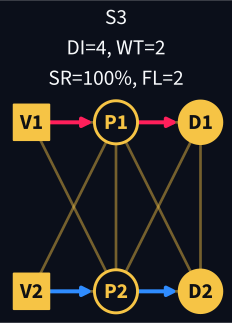
Figure 56: Route visualizations for method-selected solutions on the shared toy PDP layout. Titles report distance, total waiting, service rate, and fleet size.

Visual trade-offs:

• Each route panel corresponds to a solution chosen by one or more methods.
• Objective tuples in the titles make trade-offs explicit.
• You can compare distance, total waiting, service rate, and fleet side by side.

Decision-makers can use these visualizations alongside objective values to make informed trade-off decisions.

Method Selection Guide

Table 37: Summary of multi-objective solution methods.

Method	Best for	Guarantees	Limitations
Weighted sum	Quick exploration of trade-offs	Pareto-optimal (convex case)	Cannot find non-convex Pareto points
Epsilon-constraints	Generating complete Pareto set	Weak Pareto-optimal	Requires multiple solves; ε values must be chosen
Goal programming	Known targets or aspiration levels	Minimizes deviations	No Pareto-optimality guarantee
Lexicographic	Clear priority hierarchy	Pareto-optimal	Ignores trade-offs; lower objectives may be unconstrained

Recommended Workflow

For exploration:

1. Use \(\varepsilon\)-constraints with systematic parameter sweep to generate the full Pareto set
2. Visualize the Pareto front to understand trade-off structure

For decision-making:

3. If clear priorities exist: use lexicographic
4. If targets are known: use goal programming
5. If preferences are weights: use weighted sum (if Pareto front is convex)

Computational cost: \(\varepsilon\)-constraints requires \(O(|\varepsilon|^{n-1})\) solves for \(n\) objectives. For large problems, use weighted sum or goal programming for single-solution selection.

Use Table 37 as a quick decision checklist, then review Section 19.4 for the final summary.

Key Takeaways

Core concepts:

• Pareto optimality is the fundamental solution concept when objectives conflict
• Criterion space (objective values) vs design space (decision variables)
• Non-dominated solutions form the Pareto front

Solution techniques:

• Weighted sum: Fast but cannot find non-convex Pareto points
• \(\varepsilon\)-Constraints: Systematic but computationally expensive
• Goal programming: Intuitive (targets) but no Pareto guarantee
• Lexicographic: Strict priorities, no compromise

Practical advice:

Method Selection Depends on Context

• Convex problems: Weighted sum is efficient
• Non-convex problems: Use \(\varepsilon\)-constraints or lexicographic
• Known targets: Goal programming is natural
• Strict priorities: Lexicographic method

Normalization matters: When objectives have different units/scales, normalize before applying weighted methods.

Real-world workflow: Generate Pareto set first (exploration), then select based on stakeholder preferences (decision-making).

References

Ahuja, Ravindra K., Thomas L. Magnanti, and James B. Orlin. 1993. Network Flows: Theory, Algorithms, and Applications. Prentice Hall.

Arora, Jasbir S. 2017. “Multi-Objective Optimum Design Concepts and Methods.” In Introduction to Optimum Design, 4th ed. Elsevier. https://doi.org/10.1016/B978-0-12-800806-5.00018-4.

Boeing, Geoff. 2017. “OSMnx: New Methods for Acquiring, Constructing, Analyzing, and Visualizing Complex Street Networks.” Computers, Environment and Urban Systems 65: 126–39. https://doi.org/10.1016/j.compenvurbsys.2017.05.004.

Brown, Gerald G., and Robert F. Dell. 2007. “Formulating Integer Linear Programs: A Rogues’ Gallery.” INFORMS Transactions on Education 7 (2): 153–59.

Caramia, Massimiliano, and Paolo Dell’Olmo. 2008. Multi-Objective Management in Freight Logistics. Springer.

Chang, Kuang-Hua. 2015. “Multiobjective Optimization and Advanced Topics.” In Design Theory and Methods Using CAD/CAE. Elsevier. https://doi.org/10.1016/B978-0-12-398512-5.00005-0.

Chankong, Vira, and Yacov Y. Haimes. 1983. Multiobjective Decision Making: Theory and Methodology. Elsevier.

Clarke, G., and J. W. Wright. 1964. “Scheduling of Vehicles from a Central Depot to a Number of Delivery Points.” Operations Research 12 (4): 568–81.

Croxton, Keely L., Bernard Gendron, and Thomas L. Magnanti. 2003. “A Comparison of Mixed-Integer Programming Models for Nonconvex Piecewise Linear Cost Minimization Problems.” Management Science 49 (9): 1268–73. https://doi.org/10.1287/mnsc.49.9.1268.16570.

Dantzig, George B., and John H. Ramser. 1959a. “The Truck Dispatching Problem.” Management Science 6 (1): 80–91.

Dantzig, George B., and John H. Ramser. 1959b. “The Truck Dispatching Problem.” Management Science 6 (1): 80–91.

DHL Express. 2026. Service & Rate Guide 2026: Netherlands. PDF. https://www.dhlexpress.nl/sites/default/files/content/Netherlands%20English%20SARG26%20Full%20DEF.pdf.

Dijkstra, Edsger W. 1959. “A Note on Two Problems in Connexion with Graphs.” Numerische Mathematik 1: 269–71.

FedEx. 2026. Information on Your Rates and Shipments: Applicable in the Netherlands from 5 January 2026. PDF. https://www.fedex.com/content/dam/fedex/international/rates/new-offer-rates-domestic-en-nl.pdf.

Gendreau, Michel, Alain Hertz, and Gilbert Laporte. 1994. “A Tabu Search Heuristic for the Vehicle Routing Problem.” Management Science 40 (10): 1276–90.

Geoffrion, Arthur M. 1968. “Proper Efficiency and the Theory of Vector Maximization.” Journal of Mathematical Analysis and Applications 22 (3): 618–30.

Golden, Bruce L., Arjang A. Assad, Leon Levy, and Frederic G. Gheysens. 1984. “The Fleet Size and Mix Vehicle Routing Problem.” Computers & Operations Research 11 (1): 49–66.

Hitchcock, Frank L. 1941. “The Distribution of a Product from Several Sources to Numerous Localities.” Journal of Mathematics and Physics 20 (1-4): 224–30.

Lalla-Ruiz, Eduardo, and Stefan Voß. 2020. “A POPMUSIC Approach for the Multi-Depot Cumulative Capacitated Vehicle Routing Problem.” Optimization Letters 14 (3): 671–91.

Maffioli, Federico, and Anna Sciomachen. 2015. Chapter 2: Multi-Objective Optimization. PDF.

Miettinen, Kaisa. 1994. On the Methodology of Multiobjective Optimization with Applications. University of Jyväskylä.

Miller, Clair E., Albert W. Tucker, and Richard A. Zemlin. 1960. “Integer Programming Formulation of Traveling Salesman Problems.” Journal of the ACM 7 (4): 326–29.

Montoya-Torres, Jairo R., Julián López Franco, Santiago Nieto Isaza, Heriberto Felizzola Jiménez, and Nilson Herazo-Padilla. 2015. “A Literature Review on the Vehicle Routing Problem with Multiple Depots.” Computers & Industrial Engineering 79: 115–29.

Munson, Charles L., and Meir J. Rosenblatt. 1998. “Theories and Realities of Quantity Discounts: An Exploratory Study.” Production and Operations Management 7 (4): 352–69. https://doi.org/10.1111/j.1937-5956.1998.tb00127.x.

Murray, Chase C., and Amanda G. Chu. 2015. “The Flying Sidekick Traveling Salesman Problem: Optimization of Drone-Assisted Parcel Delivery.” Transportation Research Part C: Emerging Technologies 54: 86–109.

National Motor Freight Traffic Association. 2026. Freight Classification Development Council Procedures 2026. PDF. https://nmfta.org/wp-content/media/2026/01/FCDC-Procedures-2026.pdf.

OpenStreetMap Foundation. 2026. “OpenStreetMap Copyright and License.” https://www.openstreetmap.org/copyright.

Psaraftis, Harilaos N. 1980. “A Dynamic Programming Solution to the Single Vehicle Many-to-Many Immediate Request Dial-a-Ride Problem.” Transportation Science 14 (2): 130–54.

Solomon, Marius M. 1987a. “Algorithms for the Vehicle Routing and Scheduling Problems with Time Window Constraints.” Operations Research 35 (2): 254–65.

Solomon, Marius M. 1987b. “Algorithms for the Vehicle Routing and Scheduling Problems with Time Window Constraints.” Operations Research 35 (2): 254–65.

Sudhoff, Scott. 2007. Lecture 9: Multi-Objective Optimization. PDF slides.

Williams, Paul. 2013. Model Building in Mathematical Programming. 5th ed. Wiley.

Travel Models: Rotterdam-Zuid

Case

From demand modeling to route assignment

17

Why This Case Matters

Rotterdam-Zuid is a dense urban area where freight, commuters, bikes, and public transport share limited road capacity. Small assumptions in travel times quickly change network-level outcomes.

Modeling Principle

Use the same data backbone from demand to assignment: zones -> OD demand -> route costs -> assignment.

Planning Pipeline

graph LR
  A["Land-use and socio-demographics"] --> B["Trip generation"]
  B --> C["Trip distribution (OD matrix)"]
  C --> D["Mode split"]
  D --> E["Route assignment on road graph"]
  E --> F["Link loads and KPIs"]

Figure 57: Travel-model pipeline for Rotterdam-Zuid.

Study Area Snapshot

Figure 58: Illustrative street context for mixed traffic operations.

Representative zones for this lecture example:

• Feijenoord
• IJsselmonde
• Charlois
• Centrum

Core KPIs:

• total travel time (minutes),
• average OD generalized cost,
• overloaded links (count).

Integer Network for Classroom Computation

The teaching network uses integer arc times (minutes) so path totals are easy to verify mentally.

Arc	Time
Feijenoord -> Centrum	7
Feijenoord -> Charlois	4
Charlois -> Centrum	5
IJsselmonde -> Feijenoord	6
IJsselmonde -> Charlois	5
IJsselmonde -> Centrum	11

OD Demand Matrix (Trips per Peak Hour)

Origin  Destination	Centrum	Charlois
Feijenoord	120	80
IJsselmonde	140	90

All entries are integers and intentionally small for hand checks.

Model Block 1: Trip Distribution

Use a gravity-style form:

\[ T_{ij} = K_i O_i \frac{D_j F(c_{ij})} {\sum_{m} D_m F(c_{im})} \]

For this lecture section, calibrated factors are precomputed and rounded to integer trip totals before assignment.

Model Block 2: Mode Split

Multinomial logit for mode choice:

\[ P_{ij}^{(m)} = \frac{\exp\left(-\theta C_{ij}^{(m)}\right)} {\sum_{r \in \mathcal{M}} \exp\left(-\theta C_{ij}^{(r)}\right)} \]

Route assignment in this deck focuses on the car submatrix after mode-split.

Model Block 3: Route Assignment

Shortest-path assignment for each OD pair:

\[ \min \sum_{(u,v)\in\mathcal{E}} c_{uv} x_{uv}^{ij} \]

subject to flow conservation at every node for each OD pair \((i,j)\).

Because all arc costs are integers, assigned path costs are integer sums.

Example Route Costs (Computed on the Teaching Graph)

OD pair	Best path	Cost
Feijenoord -> Centrum	Feijenoord -> Centrum	7
IJsselmonde -> Centrum	IJsselmonde -> Centrum	11
IJsselmonde -> Charlois	IJsselmonde -> Charlois	5
Feijenoord -> Charlois	Feijenoord -> Charlois	4

Policy Questions This Model Answers

1. Which links are critical under peak demand growth?
2. How sensitive are route choices to +1 to +3 minute disruptions?
3. Which infrastructure upgrades produce the highest travel-time reduction?

References

Ahuja, Ravindra K., Thomas L. Magnanti, and James B. Orlin. 1993. Network Flows: Theory, Algorithms, and Applications. Prentice Hall.

Arora, Jasbir S. 2017. “Multi-Objective Optimum Design Concepts and Methods.” In Introduction to Optimum Design, 4th ed. Elsevier. https://doi.org/10.1016/B978-0-12-800806-5.00018-4.

Boeing, Geoff. 2017. “OSMnx: New Methods for Acquiring, Constructing, Analyzing, and Visualizing Complex Street Networks.” Computers, Environment and Urban Systems 65: 126–39. https://doi.org/10.1016/j.compenvurbsys.2017.05.004.

Brown, Gerald G., and Robert F. Dell. 2007. “Formulating Integer Linear Programs: A Rogues’ Gallery.” INFORMS Transactions on Education 7 (2): 153–59.

Caramia, Massimiliano, and Paolo Dell’Olmo. 2008. Multi-Objective Management in Freight Logistics. Springer.

Chang, Kuang-Hua. 2015. “Multiobjective Optimization and Advanced Topics.” In Design Theory and Methods Using CAD/CAE. Elsevier. https://doi.org/10.1016/B978-0-12-398512-5.00005-0.

Chankong, Vira, and Yacov Y. Haimes. 1983. Multiobjective Decision Making: Theory and Methodology. Elsevier.

Clarke, G., and J. W. Wright. 1964. “Scheduling of Vehicles from a Central Depot to a Number of Delivery Points.” Operations Research 12 (4): 568–81.

Croxton, Keely L., Bernard Gendron, and Thomas L. Magnanti. 2003. “A Comparison of Mixed-Integer Programming Models for Nonconvex Piecewise Linear Cost Minimization Problems.” Management Science 49 (9): 1268–73. https://doi.org/10.1287/mnsc.49.9.1268.16570.

Dantzig, George B., and John H. Ramser. 1959a. “The Truck Dispatching Problem.” Management Science 6 (1): 80–91.

Dantzig, George B., and John H. Ramser. 1959b. “The Truck Dispatching Problem.” Management Science 6 (1): 80–91.

DHL Express. 2026. Service & Rate Guide 2026: Netherlands. PDF. https://www.dhlexpress.nl/sites/default/files/content/Netherlands%20English%20SARG26%20Full%20DEF.pdf.

Dijkstra, Edsger W. 1959. “A Note on Two Problems in Connexion with Graphs.” Numerische Mathematik 1: 269–71.

FedEx. 2026. Information on Your Rates and Shipments: Applicable in the Netherlands from 5 January 2026. PDF. https://www.fedex.com/content/dam/fedex/international/rates/new-offer-rates-domestic-en-nl.pdf.

Gendreau, Michel, Alain Hertz, and Gilbert Laporte. 1994. “A Tabu Search Heuristic for the Vehicle Routing Problem.” Management Science 40 (10): 1276–90.

Geoffrion, Arthur M. 1968. “Proper Efficiency and the Theory of Vector Maximization.” Journal of Mathematical Analysis and Applications 22 (3): 618–30.

Golden, Bruce L., Arjang A. Assad, Leon Levy, and Frederic G. Gheysens. 1984. “The Fleet Size and Mix Vehicle Routing Problem.” Computers & Operations Research 11 (1): 49–66.

Hitchcock, Frank L. 1941. “The Distribution of a Product from Several Sources to Numerous Localities.” Journal of Mathematics and Physics 20 (1-4): 224–30.

Lalla-Ruiz, Eduardo, and Stefan Voß. 2020. “A POPMUSIC Approach for the Multi-Depot Cumulative Capacitated Vehicle Routing Problem.” Optimization Letters 14 (3): 671–91.

Maffioli, Federico, and Anna Sciomachen. 2015. Chapter 2: Multi-Objective Optimization. PDF.

Miettinen, Kaisa. 1994. On the Methodology of Multiobjective Optimization with Applications. University of Jyväskylä.

Miller, Clair E., Albert W. Tucker, and Richard A. Zemlin. 1960. “Integer Programming Formulation of Traveling Salesman Problems.” Journal of the ACM 7 (4): 326–29.

Montoya-Torres, Jairo R., Julián López Franco, Santiago Nieto Isaza, Heriberto Felizzola Jiménez, and Nilson Herazo-Padilla. 2015. “A Literature Review on the Vehicle Routing Problem with Multiple Depots.” Computers & Industrial Engineering 79: 115–29.

Munson, Charles L., and Meir J. Rosenblatt. 1998. “Theories and Realities of Quantity Discounts: An Exploratory Study.” Production and Operations Management 7 (4): 352–69. https://doi.org/10.1111/j.1937-5956.1998.tb00127.x.

Murray, Chase C., and Amanda G. Chu. 2015. “The Flying Sidekick Traveling Salesman Problem: Optimization of Drone-Assisted Parcel Delivery.” Transportation Research Part C: Emerging Technologies 54: 86–109.

National Motor Freight Traffic Association. 2026. Freight Classification Development Council Procedures 2026. PDF. https://nmfta.org/wp-content/media/2026/01/FCDC-Procedures-2026.pdf.

OpenStreetMap Foundation. 2026. “OpenStreetMap Copyright and License.” https://www.openstreetmap.org/copyright.

Psaraftis, Harilaos N. 1980. “A Dynamic Programming Solution to the Single Vehicle Many-to-Many Immediate Request Dial-a-Ride Problem.” Transportation Science 14 (2): 130–54.

Solomon, Marius M. 1987a. “Algorithms for the Vehicle Routing and Scheduling Problems with Time Window Constraints.” Operations Research 35 (2): 254–65.

Solomon, Marius M. 1987b. “Algorithms for the Vehicle Routing and Scheduling Problems with Time Window Constraints.” Operations Research 35 (2): 254–65.

Sudhoff, Scott. 2007. Lecture 9: Multi-Objective Optimization. PDF slides.

Williams, Paul. 2013. Model Building in Mathematical Programming. 5th ed. Wiley.