Warehouse design: Block layout optimization

Almost all quality improvement comes via simplification of design, manufacturing… layout, processes, and procedures. Tom Peters

🧠 Learning objectives

• Formulate block layout problems using mathematical optimization.
• Linearize the formulation.
• Discuss formulation trade-offs and caveats.

Introduction

Most facility layouts can be viewed at two levels:

• Block layout (macro flows) (location, shape, and size of each planning department)
• Detailed layout (micro flows) (exact location of equipment, work benches, and storage areas within each department).

Goal: Develop and evaluate alternative block layouts quantitatively.

The generation and evaluation of a number of layout alternatives is a critical step in the facilities planning process, since the layout selected will serve to establish the material flow patterns and physical relationships between activities. Recognizing that the layout ultimately selected will be either chosen from or based on one of the alternatives generated, it is important for the facilities planner to be both creative and comprehensive in generating a reasonable number of layout alternatives.

Most facility layouts can be viewed at two levels: The block layout (which shows the location, shape, and size of each planning department) and the detailed layout (which shows the exact location of all equipment, work benches, and storage areas within each department). The block layout is concerned primarily with the “macro” flows in the facility, while the detailed layout is often concerned with the “micro” flows. For the facility layout to be complete and effective, both the block layout and the detailed layout need to be developed and evaluated carefully. Although some of the models and techniques we show in this chapter can be applied to detailed layouts as well, our focus is primarily on quantitative methods for developing and evaluating alternative block layouts.

— Facilities Planning (Tompkins 2010, 291–92).

The layout planning project

Which comes first:

• MHS or facility layout?
  • Both! The MHS influences the facility layout and vice versa.
  • Design alternative layout plans matched with appropriate handling systems.
• Block layout or detailed layout?
  • Determine the requirements of departments and macro-flows first, then focus on their detailed layouts.

Two questions frequently arise in a layout planning project: Which comes first, the material handling system or the facility layout? Which comes first, the block layout or the detailed layout?

Many believe the layout should be designed first and the material handling system developed afterward. Yet material handling decisions can significantly affect layout effectiveness. Centralized versus decentralized work-in-process storage, fixed-path versus variable-path handling, unit loads versus one-piece flow, the degree of automation, and the type or level of inventory and material control all affect requirements for space, equipment, personnel, and proximity.

Conventional wisdom suggests addressing handling after finalizing the layout. However, if materials cannot flow directly from department A to department B, work-in-process storage is required in A, B, and/or elsewhere. A centralized storage system can change the flow pattern and eliminate the need to place A next to B. Lean manufacturing offers another alternative by creating cells so parts flow one at a time between adjacent workstations, eliminating intermediate storage and reducing handling distances and batching delays.

The “layout first” approach can also reflect a misapplication of the “handling less is best” adage. In one-piece flow, parts are handled more times than in batching, yet one-piece flow is often preferable because batching causes delay. Handling must therefore be evaluated by its effects on work-in-process inventory, throughput time, and operator travel and handling time.

Which comes first? Both. The layout and handling system should be designed simultaneously. Because the combined problem is complex, develop alternative layout plans and design an appropriate handling system, at least conceptually, for each. The preferred layout is the one resulting from consideration of the system as a whole.

For the second question, first obtain basic requirements for each department, such as space requirements and shape constraints, and then develop alternative block layouts. Once the desirable block layout is identified, develop a detailed layout for each department. The process is iterative, and starting with department information and macro flows is often practical.

— Facilities Planning (Tompkins 2010, 292–94).

Algorithmic approach: MIP (by Montreuil 1991)

Assumptions:

• All departments are assumed to be rectangular (centroid and length/width fully define location and shape).
• Department dimensions are treated as parameters.
• Distance-based objective where \(d_{ij}\) is the rectilinear distance between the centroids of departments \(i\) and \(j\).

Department \(i\) at (centroid) coordinate (\(\alpha_i, \beta_i)\) with length \(x_i^{\mathrm{right}} - x_i^{\mathrm{left}}\) and width \(y_i^{\mathrm{top}} - y_i^{\mathrm{bottom}}\) within a building of length \(B_x\) and width \(B_y\)

Using the continuous representation, the facility layout problem may be formulated as a mixed integer programming (MIP) problem if all the departments are assumed to be rectangular. Recall that, with rectangular departments, just the centroid and the length (or width) of a department fully define its location and shape. Although an alternate objective may be used, the model we show here assumes a distance-based objective (given by Equation 6.1) with \(d_{ij}\) defined as the rectilinear distance between the centroids of departments \(i\) and \(j\). Generally speaking, models based on mathematical programming are regarded as construction-type layout models since there is no need to enter an initial layout. However, as we discuss later, such models may also be used to improve a given layout.

The model we show here is based on the one presented by Montreuil. A similar model is also presented by Heragu and Kusiak, where the department dimensions are treated as parameters with known values instead of decision variables. Assuming that all department dimensions are given and fixed is appropriate in “machine layout” problems, where each “department” represents the rectangular “footprint” of a machine. Note that, with such an approach, the layout model is actually used as a two-dimensional “packing” algorithm to determine the locations of rectangular objects with known shapes. Aside from possible differences in the objective function, such a packing problem is also known as the “two-dimensional bin packing” problem.

— Facilities Planning (Tompkins 2010, sec. 6.4.6, p. 327).

Tompkins et al. explicitly state that their inspectable formulation is based on Montreuil’s model (Montreuil 1991). The symbols on this slide are the course transcription of the Tompkins formulation, not a verbatim transcription from the inaccessible Montreuil article.

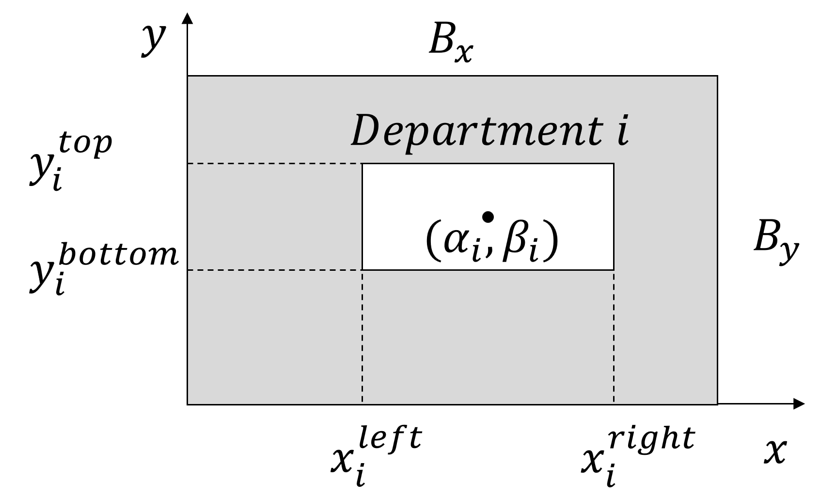
MIP as a two-dimensional packing model

The layout model is a 2D “packing” algorithm to determine the locations of rectangular objects with known shapes. Such a packing problem is also known as the “two-dimensional bin packing” problem.

Using the continuous representation, the facility layout problem may be formulated as a mixed integer programming (MIP) problem if all the departments are assumed to be rectangular. Recall that, with rectangular departments, just the centroid and the length (or width) of a department fully define its location and shape. Although an alternate objective may be used, the model we show here assumes a distance-based objective (given by Equation 6.1) with \(d_{ij}\) defined as the rectilinear distance between the centroids of departments \(i\) and \(j\). Generally speaking, models based on mathematical programming are regarded as construction-type layout models since there is no need to enter an initial layout. However, as we discuss later, such models may also be used to improve a given layout.

The model we show here is based on the one presented by Montreuil. A similar model is also presented by Heragu and Kusiak, where the department dimensions are treated as parameters with known values instead of decision variables. Assuming that all department dimensions are given and fixed is appropriate in “machine layout” problems, where each “department” represents the rectangular “footprint” of a machine. Note that, with such an approach, the layout model is actually used as a two-dimensional “packing” algorithm to determine the locations of rectangular objects with known shapes. Aside from possible differences in the objective function, such a packing problem is also known as the “two-dimensional bin packing” problem.

— Facilities Planning (Tompkins 2010, 327).

Parameters

Table 1: MIP model parameters

Symbol	Description
\(m\)	number of departments
\(f_{ij}\)	flow from dept. \(i\) to dept. \(j\) (n. of unit loads moved per unit time)
\(c_{ij}\)	cost of moving a unit load one distance unit from dept. \(i\) to dept. \(j\)
\(B_x\)	building length (measured along the x-coordinate)
\(B_y\)	building width (measured along the y-coordinate)
\(A_i\)	area of dept. \(i\)
\(L_i^{\mathrm{LB}}\)	lower limit on the length of dept. \(i\)
\(L_i^{\mathrm{UB}}\)	upper limit on the length of dept. \(i\)
\(W_i^l\)	lower limit on the width of dept. \(i\)
\(W_i^{\mathrm{UB}}\)	upper limit on the width of dept. \(i\)
\(M\)	large number (if needed)

Consider first the distance-based objective. Let \(m\) denote the number of departments, \(f_{ij}\) denote the flow from department \(i\) to department \(j\) (expressed in number of unit loads moved per unit time), and \(c_{ij}\) denote the cost of moving a unit load one distance unit from department \(i\) to department \(j\). The objective is to minimize the cost per unit time for movement among the departments. Expressed mathematically, the objective can be written as \(\min z = \sum_{i=1}^{m}\sum_{j=1}^{m} f_{ij}c_{ij}d_{ij}\), where \(d_{ij}\) is the distance from department \(i\) to \(j\). In many layout algorithms, \(d_{ij}\) is measured rectilinearly between department centroids; however, it can also be measured according to a particular aisle structure (if one is specified).

— Facilities Planning (Tompkins 2010, 304).

Treating the department dimensions as decision variables, the facility layout problem may be formulated as follows. Consider first the problem parameters. Let \(B_x\) be the building length (measured along the x-coordinate), \(B_y\) be the building width (measured along the y-coordinate), \(A_i\) be the area of department \(i\), \(L_i^{\mathrm{LB}}\) be the lower limit on the length of department \(i\), \(L_i^{\mathrm{UB}}\) be the upper limit on the length of department \(i\), \(W_i^{\mathrm{LB}}\) be the lower limit on the width of department \(i\), \(W_i^{\mathrm{UB}}\) be the upper limit on the width of department \(i\), and \(M\) be a large number.

Consider next the decision variables. Let \(\alpha_i\) be the x-coordinate of the centroid of department \(i\), \(\beta_i\) be the y-coordinate of the centroid of department \(i\), \(x_i^{\mathrm{left}}\) be the x-coordinate of the left (or west) side of department \(i\), \(x_i^{\mathrm{right}}\) be the x-coordinate of the right (or east) side of department \(i\), \(y_i^{\mathrm{top}}\) be the y-coordinate of the top (or north) side of department \(i\), \(y_i^{\mathrm{bottom}}\) be the y-coordinate of the bottom (or south) side of department \(i\), \(z_{ij}^{\mathrm{x}}\) be equal to 1 if department \(i\) is strictly to the east of department \(j\) and 0 otherwise, and \(z_{ij}^{\mathrm{y}}\) be equal to 1 if department \(i\) is strictly to the north of department \(j\) and 0 otherwise.

Note that department \(i\) would be strictly to the east of department \(j\) if and only if \(x_j^{\mathrm{right}} \leq x_i^{\mathrm{left}}\). Likewise, department \(i\) would be strictly to the north of department \(j\) if and only if \(y_j^{\mathrm{top}} \leq y_i^{\mathrm{bottom}}\). Two departments are guaranteed not to overlap if they are “separated” along either the x-coordinate (i.e., one of the departments is strictly to the east of the other) or the y-coordinate (i.e., one of the departments is strictly to the north of the other). Of course, it is possible that two departments are separated along both the x- and y-coordinates.

— Facilities Planning (Tompkins 2010, 327–28).

Variables

Table 2: MIP model variables

Symbol	Description
\(\alpha_i\)	x-coordinate of the centroid of dept. \(i\)
\(\beta_i\)	y-coordinate of the centroid of dept. \(i\)
\(x_i^{\mathrm{left}}\)	x-coordinate of the left (or west) side of dept. \(i\)
\(x_i^{\mathrm{right}}\)	x-coordinate of the right (or east) side of dept. \(i\)
\(y_i^{\mathrm{bottom}}\)	y-coordinate of the bottom (or south side) of dept. \(i\)
\(y_i^{\mathrm{top}}\)	y-coordinate of the top (or north side) of dept. \(i\)
\(z^{\mathrm{x}}_{ij}\)	1 if dept. \(i\) is strictly to the east of dept. \(j\); 0 otherwise
\(z^{\mathrm{y}}_{ij}\)	1 if dept. \(i\) is strictly to the north of dept. \(j\); 0 otherwise

Consider next the decision variables. Let \(\alpha_i\) be the x-coordinate of the centroid of department \(i\), \(\beta_i\) be the y-coordinate of the centroid of department \(i\), \(x_i^{\mathrm{left}}\) be the x-coordinate of the left (or west) side of department \(i\), \(x_i^{\mathrm{right}}\) be the x-coordinate of the right (or east) side of department \(i\), \(y_i^{\mathrm{top}}\) be the y-coordinate of the top (or north) side of department \(i\), \(y_i^{\mathrm{bottom}}\) be the y-coordinate of the bottom (or south) side of department \(i\), \(z_{ij}^{\mathrm{x}}\) be equal to 1 if department \(i\) is strictly to the east of department \(j\) and 0 otherwise, and \(z_{ij}^{\mathrm{y}}\) be equal to 1 if department \(i\) is strictly to the north of department \(j\) and 0 otherwise.

— Facilities Planning (Tompkins 2010, 327–28).

Variable relationships

Note that:

1. Dept. \(i\) is strictly to the east of dept. \(j\) \(\iff\) \(x_j^{\mathrm{right}} \leq x_i^{\mathrm{left}}\).
2. Dept. \(i\) is strictly to the north of dept. \(j\) \(\iff\) \(y_j^{\mathrm{top}} \leq y_i^{\mathrm{bottom}}\).
3. Two departments are guaranteed not to overlap if they are “separated” along either the x-coordinate (i.e., 1) or y-coordinate (i.e., 2).
4. Two departments can be separated along both the x- and y-coordinates.

Note that department \(i\) would be strictly to the east of department \(j\) if and only if \(x_j^{\mathrm{right}} \leq x_i^{\mathrm{left}}\). Likewise, department \(i\) would be strictly to the north of department \(j\) if and only if \(y_j^{\mathrm{top}} \leq y_i^{\mathrm{bottom}}\). Two departments are guaranteed not to overlap if they are “separated” along either the x-coordinate (i.e., one of the departments is strictly to the east of the other) or the y-coordinate (i.e., one of the departments is strictly to the north of the other). Of course, it is possible that two departments are separated along both the x- and y-coordinates.

— Facilities Planning (Tompkins 2010, 327–28).

Objective function

Minimize the cost per unit time for movement among the departments: the sum of rectilinear distances between departments \(d_{ij} = |\alpha_i - \alpha_j| + |\beta_i - \beta_j|\).

\[ \min \sum_{i}{\sum_{j}{f_{ij}c_{ij}(|\alpha_i - \alpha_j| + |\beta_i - \beta_j|)}} \]

Note that:

• Costs \(c_{ij}\) are implicitly assumed to be
  1. independent of the utilization of the handling equipment, and
  2. linearly related to the length of the move.
• If \(c_{ij}\) values do not satisfy (1) and (2), one may set \(c_{ij} = 1\) and focus only on total unit load travel in the facility (i.e., \(f_{ij}d_{ij}\)).
• \(c_{ij}\) may represent relative “weights” (based on unit load attributes such as size, weight, bulkiness, etc.) and minimize the weighted sum of unit load travel in the facility.

Layout algorithms can also be classified according to their objective functions. There are two basic objectives: one aims at minimizing the sum of flows times distances, while the other aims at maximizing an adjacency score. Generally speaking, the former, that is, the “distance-based” objective—which is similar to the classical quadratic assignment problem (QAP) objective—is more suitable when the input data is expressed as a from-to chart, and the latter, that is, the “adjacency-based” objective, is more suitable for a relationship chart.

Consider first the distance-based objective. Let \(m\) denote the number of departments, \(f_{ij}\) denote the flow from department \(i\) to department \(j\) (expressed in number of unit loads moved per unit time), and \(c_{ij}\) denote the cost of moving a unit load one distance unit from department \(i\) to department \(j\). The objective is to minimize the cost per unit time for movement among the departments. Expressed mathematically, the objective can be written as \(\min z = \sum_{i=1}^{m}\sum_{j=1}^{m} f_{ij}c_{ij}d_{ij}\), where \(d_{ij}\) is the distance from department \(i\) to \(j\). In many layout algorithms, \(d_{ij}\) is measured rectilinearly between department centroids; however, it can also be measured according to a particular aisle structure (if one is specified).

Note that the \(c_{ij}\) values are implicitly assumed to be independent of the utilization of the handling equipment, and they are linearly related to the length of the move. In those cases where the \(c_{ij}\) values do not satisfy the above assumptions, one may set \(c_{ij}=1\) for all \(i\) and \(j\) and focus only on total unit load travel in the facility (i.e., the product of the \(f_{ij}\) and the \(d_{ij}\) values). In some cases, it may also be possible to use the \(c_{ij}\) values as relative “weights” (based on unit load attributes such as size, weight, bulkiness, etc.) and minimize the weighted sum of unit load travel in the facility.

— Facilities Planning (Tompkins 2010, 304).

Constraints: Dimensions within bounds

The length and width of each department are within the specified bounds:

\[ \begin{align} L_i^{\mathrm{LB}} \leq (x_i^{\mathrm{right}} - x_i^{\mathrm{left}}) \leq L_{i}^{\mathrm{UB}} & \quad \text{for all} \; i \\ W_i^l \leq (y_i^{\mathrm{top}} - y_i^{\mathrm{bottom}}) \leq W_{i}^{\mathrm{UB}} & \quad \text{for all} \; i \\ \end{align} \]

Constraint sets 6.6 and 6.7 ensure that each department’s length and width lie within specified bounds. Constraint set 6.8 expresses department area and is the model’s only nonlinear constraint. Constraint sets 6.9 and 6.10 define the department sides properly and locate the department within the building in the x and y directions. Constraint sets 6.11 and 6.12 define the centroid coordinates.

Constraint set 6.13 ensures that department \(i\) is strictly east of department \(j\) if \(z_{ij}^{\mathrm{x}}=1\); when the binary variable is zero, the constraint is inactive. Constraint set 6.14 serves the same purpose in the y direction. Constraint set 6.15 prevents overlap by forcing at least one east–west or north–south separation. Constraint sets 6.16 and 6.17 impose nonnegativity, while constraint set 6.18 designates the binary variables.

— Facilities Planning (Tompkins 2010, 328–29).

Constraints: Area of department

The area requirement of each department:

\[ \begin{align} (x_i^{\mathrm{right}} - x_i^{\mathrm{left}})(y_i^{\mathrm{top}} - y_i^{\mathrm{bottom}}) = A_i & \quad \text{for all} \; i \end{align} \]

Strictly, the area constraint is a nonlinear (bilinear) constraint. Solvers such as Gurobi can handle such constraints directly (as a MIQCP problem), but they may be difficult to solve. We will show later how to linearize this constraint.

The objective function given by Equation 6.5 is the distance-based objective shown earlier as Equation 6.1. Constraint sets 6.6 and 6.7, respectively, ensure that the length and width of each department are within the specified bounds. The area requirement of each department is expressed through constraint set 6.8, which comprises the only nonlinear constraints in the model. Constraint sets 6.9 and 6.10 ensure that the department sides are defined properly and that each department is located within the building in the x and y directions, respectively. Constraint sets 6.11 and 6.12, respectively, define the x- and y-coordinates of the centroid of each department.

Due to constraint set 6.8, the above model is nonlinearly constrained. Furthermore, the objective function contains the absolute value operator. There are alternative schemes one may employ to approximate constraint 6.8 via a linear function. In [45], the department area is controlled through its perimeter (which is a linear function of the length and width of the department) and constraint sets 6.6 and 6.7.

— Facilities Planning (Tompkins 2010, eq. 6.8 and pp. 328–329).

Tompkins et al.’s internal reference [45] is retained because it is part of the printed excerpt. It identifies the source discussed by the textbook; it is not a substitution made in these notes.

In the default setting of -1 or if the NonConvex parameter is set to 2, Gurobi will accept arbitrary quadratic constraints and attempt to solve the resulting model using the appropriate algorithm.

— Gurobi Optimizer Reference Manual: Constraints (Gurobi Optimization, LLC, n.d., heading “Quadratic Constraints”).

Bilinear constraints are a special case of non-convex quadratic constraints, and the algorithms Gurobi uses to handle the latter are also well suited to solving bilinear programming problems.

— Gurobi Optimizer Reference Manual: Constraints (Gurobi Optimization, LLC, n.d., heading “Quadratic Constraints”).

The displayed equality is exact area: length times width must equal \(A_i\). Solver acceptance does not imply that the nonconvex model will be easy to solve. Tompkins et al.’s perimeter formulation is a linear approximation; it does not preserve the exact area equality.

Constraints: Proper department sizes

Department sides are defined properly and located within the building in the x and y directions:

\[ \begin{align} 0 \leq x_i^{\mathrm{left}} \leq x_i^{\mathrm{right}} \leq B_x & \quad \text{for all} \; i \\ 0 \leq y_i^{\mathrm{bottom}} \leq y_i^{\mathrm{top}} \leq B_y & \quad \text{for all} \; i \\ \end{align} \]

Constraint sets 6.9 and 6.10 ensure that the department sides are defined properly and that each department is located within the building in the x and y directions, respectively.

— Facilities Planning (Tompkins 2010, eqs. 6.9–6.10, pp. 328–329).

The inequalities place the left side before the right side between 0 and \(B_x\); the corresponding y inequalities place the bottom before the top between 0 and \(B_y\).

Constraints: Centroid coordinates

Define the centroid of each department based on x and y coordinates.

\[ \begin{align} \alpha_i = 0.5x_i^{\mathrm{left}} + 0.5x_i^{\mathrm{right}} & \quad \text{for all} \; i \\ \beta_i = 0.5y_i^{\mathrm{bottom}} + 0.5y_i^{\mathrm{top}} & \quad \text{for all} \; i \\ \end{align} \]

Constraint sets 6.11 and 6.12, respectively, define the x- and y-coordinates of the centroid of each department.

— Facilities Planning (Tompkins 2010, eqs. 6.11–6.12, pp. 328–329).

Each equality is a midpoint: the x centroid is the average of the left and right sides, and the y centroid is the average of the bottom and top sides.

Constraints: Non-overlapping departments

The department \(i\) is strictly to the east of department \(j\) if \(z_{ij}^{\mathrm{x}}=1\):

\[ \begin{align} x_j^{\mathrm{right}} \leq x_i^{\mathrm{left}} + M(1- z_{ij}^{\mathrm{x}}) & \quad \text{for all} \; i \; \text{and} \; j,\; i \neq j \end{align} \]

The department \(i\) is strictly to the north of department \(j\) if \(z_{ij}^{\mathrm{y}}=1\):

\[ \begin{align} y_j^{\mathrm{top}} \leq y_i^{\mathrm{bottom}} + M(1- z_{ij}^{\mathrm{y}}) & \quad \text{for all} \; i \; \text{and} \; j,\; i \neq j \end{align} \]

Departments are separated at least in the east–west or north–south direction:

\[ \begin{align} z_{ij}^{\mathrm{x}} + z_{ji}^{\mathrm{x}} + z_{ij}^{\mathrm{y}} + z_{ji}^{\mathrm{y}} \geq 1 & \quad \text{for all} \; i \; \text{and} \; j,\; i \leq j \end{align} \]

Constraint sets 6.6 and 6.7 ensure that each department’s length and width lie within specified bounds. Constraint set 6.8 expresses department area and is the model’s only nonlinear constraint. Constraint sets 6.9 and 6.10 define the department sides properly and locate the department within the building in the x and y directions. Constraint sets 6.11 and 6.12 define the centroid coordinates.

Constraint set 6.13 ensures that department \(i\) is strictly east of department \(j\) if \(z_{ij}^{\mathrm{x}}=1\); when the binary variable is zero, the constraint is inactive. Constraint set 6.14 serves the same purpose in the y direction. Constraint set 6.15 prevents overlap by forcing at least one east–west or north–south separation. Constraint sets 6.16 and 6.17 impose nonnegativity, while constraint set 6.18 designates the binary variables.

— Facilities Planning (Tompkins 2010, 328–29).

Non-overlap with indicator constraints

Indicator Constraints

The non-overlapping constraints model conditional statements (i.e., “if-then” statements): if \(z_{ij}^{\mathrm{x}}=1\), then \(x_j^{\mathrm{right}} \leq x_i^{\mathrm{left}}\). Similarly, if \(z_{ij}^{\mathrm{y}}=1\), then \(y_j^{\mathrm{top}} \leq y_i^{\mathrm{bottom}}\). These constraints ensure that departments do not overlap by enforcing separation along either the x- or y-coordinates.

If supported by the solver, you can use indicator constraints to model the relationships more compactly instead of using the big-M method. For example, the east–west separation constraint can be written as:

\[ \begin{align} z_{ij}^{\mathrm{x}}=1 \implies x_j^{\mathrm{right}} \leq x_i^{\mathrm{left}} & \quad \text{for all} \; i \; \text{and} \; j,\; i \neq j \end{align} \]

And similarly for the north–south direction. Using indicator constraints avoids the need for a large \(M\) and can improve numerical stability.

Constraint set 6.13 ensures that \(x_j^{\mathrm{right}} \leq x_i^{\mathrm{left}}\) (i.e., that department \(i\) is strictly to the east of department \(j\)) if \(z_{ij}^{\mathrm{x}} = 1\). Note that, if \(z_{ij}^{\mathrm{x}} = 0\), constraint set 6.13 is satisfied regardless of whether \(x_j^{\mathrm{right}} \leq x_i^{\mathrm{left}}\) or not. In other words, constraint set 6.13 becomes “active” only when \(z_{ij}^{\mathrm{x}} = 1\). Similarly, constraint set 6.14 ensures that \(y_j^{\mathrm{top}} \leq y_i^{\mathrm{bottom}}\) (i.e., that department \(i\) is strictly to the north of department \(j\)) if \(z_{ij}^{\mathrm{y}} = 1\).

Constraint set 6.15 ensures that no two departments overlap by forcing a separation at least in the east–west or north–south direction.

— Facilities Planning (Tompkins 2010, 328–29).

https://support.gurobi.com/hc/en-us/articles/4414392016529-How-do-I-model-conditional-statements-in-Gurobi

Constraints: Non-negativity and variables

\[ \begin{align} \alpha_i, \beta_i \geq 0 & \quad \text{for all} \; i \\ x_i^{\mathrm{left}}, x_i^{\mathrm{right}}, y_i^{\mathrm{bottom}}, y_i^{\mathrm{top}} \geq 0 & \quad \text{for all} \; i \\ z_{ij}^{\mathrm{x}}, z_{ij}^{\mathrm{y}} \in \{0,1\} & \quad \text{for all} \; i \; \text{and} \; j,\; i \neq j \end{align} \]

Lastly, constraint sets 6.16 and 6.17 represent the nonnegativity constraints, while constraint set 6.18 designates the binary variables.

— Facilities Planning (Tompkins 2010, eqs. 6.16–6.18, p. 328).

Nonnegativity keeps centroids and department-side coordinates inside the model’s geometric coordinate system. The binary domains make east/north placement a yes-or-no relationship for each distinct pair of departments.

Linearizing the absolute values

If \(f_{ij} \geq 0 \; \forall i,j\), the absolute value can be removed by introducing a positive part and negative part for each term:

\[ \alpha_i - \alpha_j = \alpha_{ij}^+ - \alpha_{ij}^- \quad \text{such that} \quad |\alpha_i - \alpha_j| = \alpha_{ij}^+ + \alpha_{ij}^- \\ \beta_i - \beta_j = \beta_{ij}^+ - \beta_{ij}^- \quad \text{such that} \quad |\beta_i - \beta_j| = \beta_{ij}^+ + \beta_{ij}^- \]

where \(\alpha_{ij}^+\), \(\alpha_{ij}^-\), \(\beta_{ij}^+\), and \(\beta_{ij}^-\) are all nonnegative variables.

Then, you can rewrite distances \(d_{ij}\) in the objective function:

\[ d_{ij} = (|\alpha_i - \alpha_j| + |\beta_i - \beta_j|) = (\alpha_{ij}^+ + \alpha_{ij}^- + \beta_{ij}^+ + \beta_{ij}^-) \]

Strictly, \(|x| \leq x^+ + x^-\), but high values of \(x^+\) and \(x^-\) will hurt the objective function (when minimizing and assuming \(f_{ij} \geq 0\)). Thus, the solver will force either value to zero.

Due to the area constraint, the model is nonlinearly constrained. Furthermore, the objective function contains the absolute value operator. There are alternative schemes one may employ to approximate the area constraint via a linear function. In Montreuil’s formulation, the department area is controlled through its perimeter (which is a linear function of the length and width of the department) and the length and width constraint sets.

Provided that \(f_{ij}\geq 0\) for all \(i\) and \(j\), the absolute values in the objective function may be removed by introducing a “positive part” and a “negative part” for each term. That is, set \(\alpha_i-\alpha_j=\alpha_{ij}^{+}-\alpha_{ij}^{-}\) and \(\beta_i-\beta_j=\beta_{ij}^{+}-\beta_{ij}^{-}\). Then \(|\alpha_i-\alpha_j|=\alpha_{ij}^{+}+\alpha_{ij}^{-}\) and \(|\beta_i-\beta_j|=\beta_{ij}^{+}+\beta_{ij}^{-}\), where \(\alpha_{ij}^{+}\), \(\alpha_{ij}^{-}\), \(\beta_{ij}^{+}\), and \(\beta_{ij}^{-}\) are all nonnegative variables. Hence the objective becomes \(\min z=\sum_i\sum_j f_{ij}c_{ij}(\alpha_{ij}^{+}+\alpha_{ij}^{-}+\beta_{ij}^{+}+\beta_{ij}^{-})\), together with equalities linking the positive and negative parts to the centroid differences.

— Facilities Planning (Tompkins 2010, 328–29).

The equality requires the optimization context, not only the difference equations. Algebraically, \(\alpha_i-\alpha_j=\alpha_{ij}^{+}-\alpha_{ij}^{-}\) with nonnegative parts gives \(|\alpha_i-\alpha_j|\leq\alpha_{ij}^{+}+\alpha_{ij}^{-}\). Because the model minimizes their sum with nonnegative coefficients \(f_{ij}c_{ij}\), any solution with both parts positive can reduce both by the same amount without changing their difference and strictly improve the objective. Therefore an optimal solution has at least one part equal to zero and the inequality is tight. This argument fails if the relevant objective coefficient is negative; if it is zero, an optimal solution exists with a tight split, but tightness is not forced.

Linearizing the area constraints

The department area can be controlled through its perimeter (which is a linear function of the length and width of the department).

Consider:

\[ \begin{align} P_i ^{\mathrm{LB}} & = \quad \text{lower bound on perimeter of department} \, i\\ P_i ^{\mathrm{UB}} & = \quad \text{upper bound on perimeter of department} \, i\\ \end{align} \]

and add the constraint:

\[ \begin{align} P_i^{\mathrm{LB}} \leq 2(x_i^{\mathrm{right}} - x_i^{\mathrm{left}} + y_i^{\mathrm{top}} − y_i^{\mathrm{bottom}})≤ P_i^{\mathrm{UB}} & \quad \text{for all} \; i \end{align} \]

The area to perimeter conversion is an approximation; note that an area can result in different perimeters.

Because of the exact area constraint, the original model is nonlinearly constrained, and its objective contains absolute values. Alternative schemes can approximate the area constraint with a linear function. In Montreuil’s formulation, department area is controlled through its perimeter, a linear function of department length and width, together with lower and upper bounds on length and width.

In the linear mixed-integer model, \(P_i^{\mathrm{LB}}\) and \(P_i^{\mathrm{UB}}\) are lower and upper perimeter limits. Department shapes and areas are thus controlled indirectly through length, width, and perimeter constraints. This replaces exact bilinear area equality with a linear approximation.

— Facilities Planning (Tompkins 2010, 328–30).

Area flexibility

Retaining some flexibility in departmental area requirements reduces the likelihood of having no feasible solutions when obstacles and/or fixed departments are present.

Example

Consider a 10x10 building and four departments with the following area requirements: A1 = 18, A2 = 20, A3 = 27, and A4 = 33 (note that 18+20+27+33= 98). Without flexible areas, fixing A2 at the northeast corner leads to infeasibility.

Figure 1: Alternative arrangements with relaxed area requirements (Tompkins 2010)

Fixed departments or obstacles can make exact rectangular areas infeasible. Consider a 10 by 10 building with four departments whose required areas are 18, 20, 27, and 33. The total requirement is less than 100, and without fixed departments many solutions exist. If the first department is fixed at the northeast corner, however, no feasible solution exists. If the area of department 3 or 4 is adjusted slightly, feasible arrangements can be constructed.

Retaining flexibility in departmental area requirements is therefore necessary for effective use of the model. A linear relaxation of exact area removes a nonlinear constraint and significantly reduces the likelihood that obstacles or fixed departments make the model infeasible. It also generally increases the number of feasible solutions.

— Facilities Planning (Tompkins 2010, 331–32).

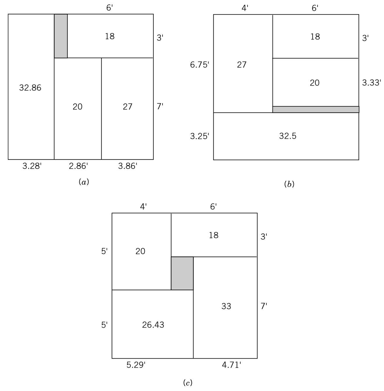
Inserting clearances between departments

To capture an “X” relationship between two departments \(i\) and \(j\), one can also insert a minimum required distance (clearance) between them.

If department \(i\) is strictly to the east of department \(j\), then \(i\) and \(j\) are separated by a minimum distance \(\Delta_{ij}^{\mathrm{x}}\) along their x-coordinates:

\[ \begin{align} x_j^{\mathrm{right}} + \Delta_{ij}^{\mathrm{x}} \leq x_i^{\mathrm{left}} + M(1- z_{ij}^{\mathrm{x}}) & \quad \text{for all} \; i \; \text{and} \; j,\; i \neq j \end{align} \]

If department \(i\) is strictly to the north of department \(j\), then \(i\) and \(j\) are separated by a minimum distance \(\Delta_{ij}^{\mathrm{y}}\) along their y-coordinates:

\[ \begin{align} y_j^{\mathrm{top}} + \Delta_{ij}^{\mathrm{y}} \leq y_i^{\mathrm{bottom}} + M(1- z_{ij}^{\mathrm{y}}) & \quad \text{for all} \; i \; \text{and} \; j,\; i \neq j \end{align} \]

Clearances should be used sparingly; they limit the number of feasible solutions.

We remarked earlier that the layout planner may represent an X relationship between departments \(i\) and \(j\) by assigning a negative value to \(f_{ij}\). However, the transformation we used earlier to linearize the model requires that \(f_{ij}\geq 0\) for all \(i\) and \(j\). While this requirement rules out the use of “negative flow” values, it does not imply that the above model cannot effectively capture an X relationship between two departments. One may insert a minimum required distance between two departments \(i\) and \(j\) by modifying constraints 6.31 and 6.32.

Let \(\Delta_{ij}^{\mathrm{x}}\) and \(\Delta_{ij}^{\mathrm{y}}\) denote the minimum required distance (or clearance) between departments \(i\) and \(j\) along the x- and y-coordinates, respectively. Such clearances should be used sparingly; otherwise, the number of feasible solutions can be very limited. Also, note that if departments \(i\) and \(j\) are separated along, say, only the x-coordinate, then the resulting clearance between them along the y-coordinate may be less than \(\Delta_{ij}^{\mathrm{y}}\).

— Facilities Planning (Tompkins 2010, 329–30).

Controlling the shape of departments

Place an upper limit on the ratio (\(R_i \geq 1\)) of department \(i\)’s longer side to its shorter side:

\[ \begin{align} (x_i^{\mathrm{right}} - x_i^{\mathrm{left}}) \leq R_i(y_i^{\mathrm{top}} - y_i^{\mathrm{bottom}}) & \quad \text{for all} \; i \\ (y_i^{\mathrm{top}} - y_i^{\mathrm{bottom}}) \leq R_i(x_i^{\mathrm{right}} - x_i^{\mathrm{left}}) & \quad \text{for all} \; i \\ \end{align} \]

Depending on which side is the longer, at most one (i.e., could be none) of the above constraints will be “binding” (i.e., hold as an equality for non-square departments).

Department shapes and areas are indirectly controlled through length, width, and perimeter constraints. Shape may also be controlled explicitly by placing an upper limit on the ratio of a department’s longer side to its shorter side. If the limit is \(R_i \geq 1\), one constraint limits length to \(R_i\) times width and another limits width to \(R_i\) times length.

Depending on which side is longer, at most one of the two constraints will be binding, or hold as an equality, for a nonsquare department. Together they prevent either orientation from becoming excessively long and narrow.

— Facilities Planning (Tompkins 2010, 329–30).

Caveats

• If too complex, terminate the branch-and-bound search when the gap (i.e., the difference between the least lower bound and the incumbent solution) is within a certain bound (e.g., 5–10%).
• Determine the north–south and east–west relationships between the departments (i.e., \(z_{ij}^{\mathrm{y}}\) and \(z_{ij}^{\mathrm{y}}\) variables) a priori by constructing a “design skeleton.” Then, the MIP model will only “pack” the departments within the building.
• There are cases where L-shaped or U-shaped departments may be more appropriate or necessary.
• The MIP model may also be used to improve a given layout (i.e., find the locations of non-fixed departments) after specifying the known dimensions and location of fixed departments and/or obstacles (i.e., \(x_i^{\mathrm{left}}\), \(x_i^{\mathrm{right}}\), \(y_i^{\mathrm{bottom}}\), \(y_i^{\mathrm{top}}\), \(\alpha_i\), and \(\beta_i\)).
  • Non-rectangular obstacles may be represented as a collection of rectangular dummy departments.

Hence, provided that the departmental area requirements need not be satisfied with precision, the optimum layout with rectangular departments can be, in theory, obtained by solving the MIP model given by Equations 6.21 through 6.37. For real-world problems, obtaining an exact solution to the above model is not straightforward due to the large number of binary variables involved. However, as further research on MIP and similar mathematical programming-based layout models is conducted, both the problem size (expressed as the number of departments) that can be tackled and the accuracy with which the department area constraints can be satisfied have been improving. Of course, faster computers and better optimization packages are also playing a role.

To use the MIP model in practice (where the number of departments can easily exceed 18), one may aim for a heuristic solution rather than the optimal solution. One obvious heuristic approach is to terminate the branch-and-bound search when the difference between the least lower bound and the incumbent solution is less than, say, 5 or 10%. The advantage of such an approach is that the resulting solution is guaranteed to be within 5 or 10% of the optimum; the primary drawback is that it may still take a substantial amount of computer time to identify such a solution.

Another possible heuristic approach is to determine the north–south and east–west relationships between the departments a priori by constructing a “design skeleton.” With such an approach, first the \(z_{ij}^{\mathrm{x}}\) and \(z_{ij}^{\mathrm{y}}\) values are determined heuristically, and the MIP model shown by Equations 6.21 through 6.37 can then be solved as a linear programming problem to “pack” the departments within the building.

There are many real-world applications where the ideal shape of a department is a rectangle. However, there are also cases where L-shaped or U-shaped departments may be more appropriate or necessary. Furthermore, if there are fixed departments or obstacles in the building, enforcing rectangular department shapes with exact area values may make it impossible to find a feasible solution (even if the continuous representation is used and the fixed departments and obstacles are rectangular).

For example, consider a 10 by 10 building and four departments with the following area requirements: \(A_1=18\), \(A_2=20\), \(A_3=27\), and \(A_4=33\). Note that the total area requirement is actually less than 100 units. If none of the departments are fixed, then the above problem obviously has many feasible solutions. However, if the first department is fixed, say, at the northeast corner of the building, then there is no feasible solution to the problem. In contrast, if the area of, say, department 3 or 4 can be slightly adjusted, then three feasible solutions can be constructed.

Thus, retaining some flexibility in departmental area requirements is necessary for the effective use of the MIP model. In fact, approximating the departmental areas through some linear relaxation of constraint 6.8 serves a dual purpose: it allows one to remove a nonlinear constraint, and at the same time it significantly reduces the likelihood of having no feasible solutions when obstacles and/or fixed departments are present. Of course, generally speaking, it also increases the number of feasible solutions.

The MIP model may also be used to improve a given layout after specifying the dimensions and location of fixed departments in the initial layout. This is accomplished simply by setting \(\alpha_i\), \(\beta_i\), \(x_i^{\mathrm{left}}\), \(x_i^{\mathrm{right}}\), \(y_i^{\mathrm{bottom}}\), and \(y_i^{\mathrm{top}}\) equal to their appropriate values for all the fixed departments and/or obstacles. Nonrectangular obstacles may be represented as a collection of rectangular dummy departments. Note that, with such an approach, the initial layout is “improved” not by exchanging department locations but rather by determining the new locations of all the nonfixed departments at once. Since such an approach does not explicitly consider “incremental” improvements to the layout and the resulting relocation costs versus material handling savings, it may not be a practical approach.

If relocation costs are significant, the layout planner may systematically fix and unfix certain subsets of the nonfixed departments and solve the MIP model several times to affect incremental changes in the layout. Alternately, the layout planner may first determine what the north–south/east–west relationships are going to be for two departments after their exchange, and then subsequently use these relationships and the above MIP model to “repack” the departments with two of them exchanged.

— Facilities Planning (Tompkins 2010, 330–31).

References

Gurobi Optimization, LLC. n.d. “Constraints — Gurobi Optimizer Reference Manual.” Accessed September 3, 2026. https://docs.gurobi.com/projects/optimizer/en/current/concepts/modeling/constraints.html.

Montreuil, Benoit. 1991. “A Modelling Framework for Integrating Layout Design and Flow Network Design.” In Material Handling ’90, edited by Robert J. Graves, Mickey R. Wilhelm, Leon F. McGinnis, and Richard E. Ward. Springer. https://doi.org/10.1007/978-3-642-84356-3_8.

Tompkins, James A., ed. 2010. Facilities Planning. 4th ed. J. Wiley.