Warehouse design and product allocation

The paper presents a mathematical model and a heuristic algorithm that jointly determine product allocation to the functional areas in the warehouse as well as the size of each area using data readily available to a warehouse manager.

— Mathematical Model for Warehouse Design and Product Allocation (Heragu et al. 2005, 327).

Learning objectives

• Differentiate the functions of the cross-docking, reserve, and forward areas.
• Formulate space allocation and product-flow assignment using mathematical optimization.
• Discuss the model’s assumptions, cost trade-offs, and constraints.

Contents

1. Functional areas and material flows
2. Model parameters and decision variables
3. Objective function and constraints

Functional areas and material flows

01

The paper presents a mathematical model and a heuristic algorithm that jointly determine product allocation to the functional areas in the warehouse as well as the size of each area using data readily available to a warehouse manager.

— Mathematical Model for Warehouse Design and Product Allocation (Heragu et al. 2005, 327).

Design model for warehouse space allocation

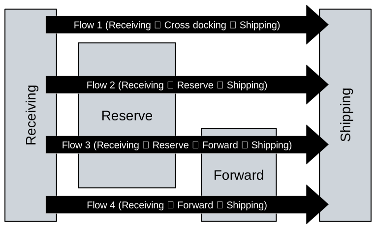
Figure 1: Typical warehouse product flow (based on Heragu 2022).

The design problem joins two decisions: select one material flow for each product and size the functional areas required by those assignments. Its objective trades annual handling cost against area-dependent storage cost. Inventory price and carrying rate help estimate EOQ and dwell time; inventory holding cost is not an additional term in the model objective.

The two primary functions of a warehouse include (1) temporary storage and protection of goods and (2) providing value added services such as fulfilment of individual customer orders, packaging of goods, after sales services, repairs, testing, inspection and assembly. To perform the above functions, the warehouse is divided into several functional areas such as reserve storage area, forward (order collation) area and cross-docking. The paper presents a mathematical model and a heuristic algorithm that jointly determine product allocation to the functional areas in the warehouse as well as the size of each area using data readily available to a warehouse manager.

— Mathematical Model for Warehouse Design and Product Allocation (Heragu et al. 2005, 327, abstract).

The next section presents a mathematical model that determines the flow to which each product must be assigned and as result, the size of the functional areas within the warehouse. It assumes the following: available total storage space is known; expected time a product spends on the shelves is known (the dwell time); cost of handling each product in each flow is known; dwell time and cost have a linear relationship; annual product demand rates are known; and storage policies and material-handling equipment are known and these affect the unit handling and storage costs.

— Mathematical Model for Warehouse Design and Product Allocation (Heragu et al. 2005, 330–31, secs. 3–4).

The dwell time is the average duration a product stays on the shelf and is assumed to be known or can be estimated by the warehouse manager. In fact, based on annual product demand \(\lambda_i\), order cost \(A_i\), price per unit load of product \(P_i\) and carrying cost rate \(r\), a simple economic order quantity (EOQ) model can be used to determine the optimal order quantity \(Q_i\), as well as the average time a unit load of product spends on the shelves. For example, since the time between two successive replenishments is \(Q_i/\lambda_i\), the average dwell time per unit load of product \(i\) is \(T_i=Q_i/(2\lambda_i)\). Note that \(Q_i/2=\lambda_iT_i\) and this value or another reasonable estimate must be used in the objective function, which minimizes the total cost of handling the average, annual loads of each product assigned to its respective area as well as the corresponding annual storage costs.

The reader should not confuse storage costs with inventory holding costs. While inventory holding costs depend only upon the value of the inventory, they are the same whether the inventory is in reserve or forward or cross-docking area. Storing costs, on the other hand, depend upon the area in which the product is stored and these costs tend to carry a premium for the cross-docking and forward areas (because these are considered prime real estate in a warehouse) and are relatively not that expensive for the reserve area. Of course, the handling costs are different (in fact, the opposite) for these areas and thus our model trades off storage costs against handling costs.

— Mathematical Model for Warehouse Design and Product Allocation (Heragu et al. 2005, 332–33, sec. 4).

Exercise 2 Role of functional areas in a warehouse

In Table 1, match each row in the “Functions” column with the appropriate Functional Area: 1) Receiving, 2) Shipping, 3) Staging for Cross-Docking, 4) Reserve, and 5) Forward.

Table 1: Matching functions to functional areas in a warehouse.

Functional Area	Function
Forward	Optimized for order collation and rapid replenishment.
Receiving	Pallet loads or individual cartons of products are received.
Shipping	Picked order items are staged and value-added services are performed.
Staging	In cross-docking, products are sorted for outbound operations.
Forward	Performs value-added operations such as labeling or kitting.
Staging	Received products are pre-sorted.
Receiving	Products are staged briefly and then moved to the shipping area (cross-docking) or the storage area.
Reserve	High-density storage equipment is used to maximize space utilization.
Forward	Smaller storage area designed for fast order picking.
Staging	Items wait temporarily before being moved to the shipping area.
Reserve	Stores bulky products for extended periods.

Subset of functional areas

• Receiving area
  • Pallet loads/individual cartons of products are received.
  • Products are staged (if necessary) for a short period and are moved either to:
    • the shipping area directly (cross-docking operation) or
    • the storage area
• Shipping area
  • Picked order items are
    • readied (e.g., shrinkwrapped, packed) and
    • staged (if necessary) for shipping

• Staging for cross-docking
  • Products are sorted and accumulated for further outbound operations.
  • Items are either
    1. put into a staging area (short period) and then moved to the shipping area or
    2. directly moved to the shipping area.
• Received products are typically presorted at suppliers’ facilities.

These are candidate functional areas, not a claim that every warehouse contains all five. A particular design may use a subset. Receiving accepts and briefly stages arrivals; shipping readies outbound orders; cross-dock staging sorts and accumulates products that move onward without reserve or forward storage.

This paper considers warehouse configurations that include a subset of the following five functional areas: receiving, shipping, staging for cross-docking operation, reserve and forward. In the receiving area, pallet loads or individual cartons of products are received. If necessary, they are staged for a short period and then moved either to the shipping area directly (cross-docking operation) or to the storage area. In the shipping area, picked order items are readied (e.g. shrink-wrapped, packed) and staged (if necessary) for shipping to the next destination. In the staging area for cross-docking, products are sorted and accumulated for further outbound operations. The reserve area is a storage area for bulky product items that typically reside in the warehouse for a relatively longer duration. Normally, the reserve area uses high-density storage equipment to achieve the goal of high space utilization. The forward area is a relatively smaller storage area typically used for fast order picking or performing value-added operations or order collation. Thus, the following material flows are possible in a warehouse: Flow 1, receiving to cross-docking to shipping; Flow 2, receiving to reserve area to shipping; Flow 3, receiving to reserve area to forward area to shipping; and Flow 4, receiving to forward area to shipping.

Flow 1 is the cross-docking operation. Upon receipt, product items are either put into a staging area for a short period and then moved to the shipping area, or directly moved to the shipping area. The received products are typically presorted at suppliers’ facilities. The operation here is simply to pass on the product to a customer or the next facility in the supply chain.

Flow 3 is also a typical warehouse operation. Products are first stored in the reserve area typically in pallet loads, broken into smaller loads (cartons or cases) and then moved to the forward area for fast order picking, order consolidation or performing value added operations.

— Mathematical Model for Warehouse Design and Product Allocation (Heragu et al. 2005, 329–30, sec. 3).

Subset of functional areas: storage

• Reserve area
  • Typically bulky product items
    • Relatively extended periods
    • Shipped as is (or with minimal “value-added” operations)
  • High-density storage equipment
  • Focus on high space utilization

• Forward area
  • Smaller storage area
  • Fast order picking
  • Value-added operations
  • Order collation

In this section, we consider warehouse configurations that include a subset of the following five functional areas: receiving, shipping, staging for cross-docking operation, reserve, and forward.

In the receiving area, pallet loads or individual cartons of products are received. If necessary, they are staged for a short period and then either moved to the shipping area directly (cross-docking operation) or to the storage area. In the shipping area, picked order items are readied (e.g., shrink-wrapped, packed) and staged (if necessary) for shipping to the next destination.

In the staging area for cross-docking, products are sorted and accumulated for further outbound operations.

Reserve area is a storage area for bulky product items that typically reside in the warehouse for a relatively longer duration. Normally, the reserve area uses high-density storage equipment to achieve the goal of high space utilization.

Forward area is a relatively smaller storage area typically used for fast order picking or performing value-added operations or order collation. Thus, the following material flows are possible in a warehouse: Flow 1: receiving to cross-docking to shipping; Flow 2: receiving to reserve area to shipping; Flow 3: receiving to reserve area to forward area to shipping; and Flow 4: receiving to forward area to shipping.

— Mathematical Model for Warehouse Design and Product Allocation (Heragu et al. 2005, 329–30).

Flows

• (Flow 1) Receiving ➤ Cross docking ➤ Shipping: Products are passed on to customers or next facility in the supply chain.
• (Flow 2) Receiving ➤ Reserve ➤ Shipping: Products are stored in the reserve area, and order-picking operation is performed as required.
• (Flow 3) Receiving ➤ Reserve ➤ Forward ➤ Shipping: Products are
  1. stored in the reserve area (typically in pallet loads),
  2. broken into smaller loads (cartons or cases), and
  3. moved to the forward area for fast order picking.
• (Flow 4) Receiving ➤ Forward ➤ Shipping: Products are put directly into the forward area for order consolidation (common in supplier warehouses).

Flow 1 is the cross-docking operation. Upon receipt, product items are either put into a staging area for a short period and then moved to the shipping area or directly moved to the shipping area. The received products are typically presorted at suppliers’ facilities. The operation here is simply to pass on the product to a customer or the next facility in the supply chain. A number of companies use this strategy for efficient operation and management of the supply chain (Editor, 1996c).

Flow 2 is a typical warehouse operation. Products are stored in the reserve area and order-picking operation is performed as required. It is assumed that typically only those items that remain in the warehouse for relatively extended periods and are shipped as is (or with minimal value-added operations) will be allocated to the reserve storage area.

Flow 3 is also a typical warehouse operation. Products are first stored in the reserve area typically in pallet loads, broken into smaller loads (cartons or cases), and then moved to the forward area for fast order picking, order consolidation, or performing value-added operations.

Flow 4 can be thought of as another form of cross-docking operation. Products are received and then directly put into the forward area to perform the order consolidation. This type of operation is usually seen in supplier warehouses or when there is a need to consolidate large orders.

— Mathematical Model for Warehouse Design and Product Allocation (Heragu et al. 2005, 330–31).

Model parameters and decision variables

02

The next section presents a mathematical model that determines the flow to which each product must be assigned and as result, the size of the functional areas within the warehouse.

— Mathematical Model for Warehouse Design and Product Allocation (Heragu et al. 2005, 330–31).

Mathematical model

Goal: Determine the product-flow assignment and the functional-area sizes within the warehouse.

Assumptions:

1. The available total storage space is known.
2. A product’s expected time on the shelves (dwell time) is known.
3. The cost of handling each product in each flow is known.
4. The dwell time and cost have a linear relationship.
5. The annual product demand rates are known.
6. The storage policies and material-handling equipment are known, and these affect the unit handling and storage costs.

Indexes (products, flows)

Table 2: MIP model indexes for products and flows

Symbol	Description
\(i\)	Number of products \(i \in \{1, 2, \dots, n\)}
\(j\)	Type of material flow; \(j \in \{1, 2, 3, 4\}\)

Model product flows

Parameters (costs, prices, EOQ, dwell time)

Table 3: MIP model parameters to calculate the EOQ

Symbol	Description
\(D_{i}\)	Annual demand rate of product \(i\) in unit loads
\(C_{i}^{\mathrm{order}}\)	Order cost for product \(i\)
\(P_i\)	Price per unit load of product \(i\)
\(C^{\mathrm{carry}}\)	Carrying cost/unit of inventory/year (%) rate
\(Q_i\)	Order quantity for product \(i\) (in unit loads)
\(T_i\)	Avg. dwell time (in years) per unit load of product \(i\)

Model product flows

The slide writes annual demand as \(D_i\); Heragu et al. use \(\lambda_i\) for the same role. \(C_i^{\mathrm{order}}\) is currency per replenishment, \(P_i\) is currency per unit load, and \(C^{\mathrm{carry}}\) is a fraction per year. Their product, \(P_iC^{\mathrm{carry}}\), is therefore a holding cost in currency per unit load per year. \(Q_i\) is the replenishment quantity, and \(T_i=Q_i/(2D_i)\) is average dwell time under the EOQ inventory-cycle assumptions.

The next section presents a mathematical model that determines the flow to which each product must be assigned and as result, the size of the functional areas within the warehouse. It assumes the following: available total storage space is known; expected time a product spends on the shelves is known (the dwell time); cost of handling each product in each flow is known; dwell time and cost have a linear relationship; annual product demand rates are known; and storage policies and material-handling equipment are known and these affect the unit handling and storage costs.

— Mathematical Model for Warehouse Design and Product Allocation (Heragu et al. 2005, 330–31, secs. 3–4).

The dwell time is the average duration a product stays on the shelf and is assumed to be known or can be estimated by the warehouse manager. In fact, based on annual product demand \(\lambda_i\), order cost \(A_i\), price per unit load of product \(P_i\) and carrying cost rate \(r\), a simple economic order quantity (EOQ) model can be used to determine the optimal order quantity \(Q_i\), as well as the average time a unit load of product spends on the shelves. For example, since the time between two successive replenishments is \(Q_i/\lambda_i\), the average dwell time per unit load of product \(i\) is \(T_i=Q_i/(2\lambda_i)\). Note that \(Q_i/2=\lambda_iT_i\) and this value or another reasonable estimate must be used in the objective function, which minimizes the total cost of handling the average, annual loads of each product assigned to its respective area as well as the corresponding annual storage costs.

— Mathematical Model for Warehouse Design and Product Allocation (Heragu et al. 2005, 332–33, sec. 4).

It is worth pausing to point out some implications of this model that will be useful in the context of warehouses. First, the average inventory over time is \(Q/2\). This means that the average time in inventory of this particular item is \(Q/(2D)\). This expression is frequently called turnover time. The inverse value is the average number of inventory turns. Note that the number of turns is not the same—indeed, is twice the value of—the number of times the item is ordered and replenished.

The obvious question to ask is what is the best quantity \(Q\) to order? To answer this we must enlarge the model by including some costs. The main costs common to inventories are the costs of reordering and the costs of holding inventory.

An order cycle is initiated by the placing of the order, which incurs cost \(c_T\). Thereafter, holding costs are accrued for inventory-time (for example, widget-years), which is the area under the inventory curve. Summing these two cost components gives the total cost of one inventory cycle: \(c_T+c_H Q^2/(2D)\). The cost per unit time is given by dividing the cost per cycle by the duration \(Q/D\) of a cycle, which gives \(c_TD/Q+c_HQ/2\). Minimizing this rate of cost gives the economic order quantity: \(Q^*=\sqrt{2Dc_T/c_H}\).

— Warehouse & Distribution Science (Bartholdi and Hackman 2019, 295–96, appendix A.1).

EOQ formula

• For a given product \(i\):
  • \(C_{i}^{\mathrm{order}}\): order cost
  • \(D_{i}\): annual demand rate
  • \(C_{i}^{\mathrm{carry}}\): inventory carrying cost rate/unit/year
  • \(P_i\): price per unit load
  • \(P_iC_{i}^{\mathrm{carry}}\): inventory carrying cost/unit/year

• The optimal order quantity is \[ Q_i = \sqrt{\frac{2D_{i}C_{i}^{\mathrm{order}}}{P_iC^{\mathrm{carry}}}} \]

• Example of EOQ calculation:
  • \(C_{i}^{\mathrm{order}}\) = $200 per order
  • \(D_{i}\) = 3,600 units/year
  • \(C_{i}^{\mathrm{carry}}\) = 25%
  • \(P_i\) = $100 per unit
  • \(P_iC_{i}^{\mathrm{carry}} = 100 \times 25\% = \$25\)/unit/year

• The optimal order quantity is:

  \[ \begin{align} Q_i = & \sqrt{\frac{2 \times 3,600 \times 200}{25}} \\ = & 240 \; \text{units}\\ \end{align} \]

Average dwell time (turnover time)

Average duration a product stays on the shelf (time between two successive replenishments).

• Known or estimated by the warehouse manager.
• Can be estimated using the EOQ¹ \(Q_{i}\) and annual demand \(D_{i}\) of product \(i\):
  1. The cycle time is \(\frac{Q_{i}}{D_{i}}\) years.
  2. The avg. dwell time is \(T_i = \frac{Q_i}{2D_{i}}\) years.
  3. The avg. n. of turns is \(\frac{1}{T_i}\).
  4. The avg. annual load is \(D_iT_i = \frac{Q_i}{2}\) units.

Example of dwell time calculation:

• \(Q_{i}\) = 240 units
• \(D_{i}\) = 3,600 units/year
• cycle time = \(\frac{240}{3,600} = \frac{1}{15} \; \text{years}\)
• Number of replenishments/reorders = 15

The avg. dwell time is:

\[ \begin{align} T_i = & \frac{240}{2 \times 3,600} = \frac{1}{\underbrace{30}_{\substack{avg. \\ turns}}} \; \text{years (3.2 weeks)}\\ \end{align} \]

The avg. annual load is

\[ \frac{Q_i}{2} = \frac{240}{2} = 120\; \text{units} \]

The dwell time is the average duration a product stays on the shelf and is assumed to be known or can be estimated by the warehouse manager. In fact, based on annual product demand \(lambda_i\), order cost \(A_i\), price per unit load of product \(P_i\), and carrying cost rate \(r\), a simple economic order quantity (EOQ) formula, \(Q_i = \sqrt{2\lambda_i A_i/(rP_i)}\), can be used to determine the optimal order quantity \(Q_i\), as well as the average time a unit load of a product spends on the shelves. For example, because the time between two successive replenishments is \(Q_i/\lambda_i\), the average dwell time per unit load of product \(i\) is \(T_i = 0.5Q_i/\lambda_i\). Note that \(0.5Q_i = \lambda_iT_i\), and this value or another reasonable estimate must be used in the objective function (8.2), which minimizes the total cost of handling the average annual loads of each product assigned to its respective area and the corresponding annual storage costs.

— Facilities Design (Heragu 2022, 289).

It is worth pausing to point out some implications of this model that will be useful in the context of warehouses. First, the average inventory over time is \(Q/2\). This means that the average time in inventory of this particular item is \(Q/(2D)\). This expression is frequently called turnover time. The inverse value is the average number of inventory turns. Note that the number of turns is not the same—indeed, is twice the value of the number of times the item is ordered and replenished.

— Warehouse & Distribution Science (Bartholdi and Hackman 2019, 295).

1. EOQ: Economic Order Quantity

Parameters (product to flow handling & storage)

Table 4: MIP model parameters

Symbol	Description
\(C_{ij}^{\mathrm{handle}}\)	Cost of handling a unit load of product \(i\) in material flow \(j\)
\(C_{ij}^{\mathrm{store}}\)	Cost of storing a unit load of product \(i\) in material flow \(j\) per year
\(\rho_{i}^{\mathrm{R}}\)	Average percentage of time a unit load of product \(i\) spends in the reserve area if product is assigned to material flow 3
\(d_i\)	Ratio of the size of the unit load in the reserve area to that in the forward area
\(q_{ij}\)	Break-bulk factor: = \(1\) if product \(i\) is assigned to material flow \(j \in \{1,2,4\}\) = \(\lceil d_i \rceil + 1\) when product \(i\) is assigned to flow \(j =3\)

Product flows and the break-bulk factor

Model product flows.

Flow 3 is the only modeled flow that changes unit-load size: reserve storage handles supplier pallet loads, while the forward area handles the resulting cartons or cases. For example, \(d_i=\frac{\text{pallet-load size}}{\text{carton-load size}}\geq1\). The ratio \(d_i\) describes the size conversion. The factor \(q_{i3}=\lceil d_i\rceil+1\) is a handling-count multiplier, not only a physical pallet-to-carton conversion factor, and the flow-3 handling and storage costs must be aggregated accordingly.

Flow 3 is also a typical warehouse operation. Products are first stored in the reserve area typically in pallet loads, broken into smaller loads (cartons or cases) and then moved to the forward area for fast order picking, order consolidation or performing value added operations.

— Mathematical Model for Warehouse Design and Product Allocation (Heragu et al. 2005, 329–30, sec. 3).

The exception is for products assigned to flow 3 because these products have different unit load sizes in the two areas encompassing flow 3. The unit load size of products assigned to flow 3 could be equal to that received from the suppliers in the reserve area, but different when handled in the forward area. This occurs because a pallet load is broken down to cases or cartons in the forward area. This is only for products assigned to flow 3. Hence, we introduce \(d_i\) to denote the ratio of the size of the unit load in the reserve area to that in the forward area and \(q_{ij}\) for \(j=3\) accounts for the fact that product \(i\) is handled \(\lceil d_i\rceil+1\) times. \(H_{ij}\) and \(C_{ij}\) should therefore correspond to aggregate handling and storage costs for \(j=3\).

— Mathematical Model for Warehouse Design and Product Allocation (Heragu et al. 2005, 332–33, sec. 4).

Storage vs. inventory holding costs

• Inventory holding costs (\(C^{\mathrm{carry}}\)) depend only on the value of the inventory.
  • Same whether the inventory is in reserve or forward or cross-docking area.
• Storage costs (\(C_{ij}^{\mathrm{store}}\)) depend on the area in which the product is stored.
  • Costs tend to carry a premium for the cross-docking and forward areas (prime real estate in a warehouse).
  • Costs tend to be cheaper for the reserve area.

The reader should not confuse storage costs with inventory holding costs. While inventory holding costs depend only on the value of the inventory, they are the same whether the inventory is in reserve or forward or cross-docking area. Storing costs, on the other hand, depend on the area in which the product is stored, and these costs tend to carry a premium for the cross-docking and forward areas (because these are considered prime real estate in a warehouse) and are relatively not that expensive for the reserve area.

— Facilities Design (Heragu 2022, 289).

Storage and handling costs

• Storage costs (\(C_{ij}^{\mathrm{store}}\)) of product \(i\) in material flow \(j\) are a function of:
  • The size of a product’s unit load.
  • Warehouse leasing/construction costs per square meter.
  • Shelving type used in each area encompassing flow \(j\).
• Handling costs (\(C_{ij}^{\mathrm{handle}}\)) of product \(i\) in material flow \(j\) are a function of:
  • Product size.
  • Product handling characteristics.
  • Material handling system used in the area(s) included in flow \(j\).

We believe much of the input data such as the type and number of products, annual demand for each, order cost, unit price, and carrying cost rate are readily available to the warehouse designer. The storage cost \(C_{ij}\) is typically a function of the size of a product’s unit load, warehouse leasing or construction costs per square foot, as well as the type of shelving used in each area encompassing flow \(j\). \(C_{ij}\) and \(H_{ij}\) for flow 3 must be aggregated to account for the fact that a pallet load could be broken down into cases or cartons. The cost of handling a unit load of product \(i\) in each flow \(j\) is a function of the product size, its handling characteristics, and the MHS used in the area(s) included in flow \(j\). Chapter 3 provides a simple formula to estimate these costs based on labor, nonlabor, and prorated capital recovery costs of the MHS. Adapting this formula to the warehouse application is left as an exercise (see Exercise 29). The model (8.2) through (8.11) can be solved optimally using available mixed-integer programming software, and even large-scale problems with 75,000 items can be solved.

— Facilities Design (Heragu 2022, 290).

Parameters (space allocation)

Table 5: MIP model parameters regarding functional area spaces

Symbol	Description
\(S^{\mathrm{total}}\)	Total available storage space
\(S_{i}\)	Space required for storing a unit load of product \(i\)
\(z^{\mathrm{CD}}\), \(z^{\mathrm{R}}\), \(z^{\mathrm{F}}\)	Levels of space available in the vertical dimension in each functional area
\(LL_{\mathrm{CD}}\), \(UL_{\mathrm{CD}}\)	Lower and upper storage space limit for the cross-docking area
\(LL_{\mathrm{F}}\), \(UL_{\mathrm{F}}\)	Lower and upper storage space limit for the forward area
\(LL_{\mathrm{R}}\), \(UL_{\mathrm{R}}\)	Lower and upper storage space limit for the reserve area

Model product flows

The source notation uses \(TS\) for total available storage space, \(S_i\) for the space required by one unit load, \(a\), \(b\), and \(c\) for the available vertical levels in cross-dock, reserve, and forward areas, and lower/upper limits for each area. The slide renames these quantities to make the area explicit. \(S^{\mathrm{total}}\) is storage space, not total building area; multiplying it by a consistent vertical-level factor gives the capacity used in the area constraints.

The next section presents a mathematical model that determines the flow to which each product must be assigned and as result, the size of the functional areas within the warehouse. It assumes the following: available total storage space is known; expected time a product spends on the shelves is known (the dwell time); cost of handling each product in each flow is known; dwell time and cost have a linear relationship; annual product demand rates are known; and storage policies and material-handling equipment are known and these affect the unit handling and storage costs.

— Mathematical Model for Warehouse Design and Product Allocation (Heragu et al. 2005, 330–31, secs. 3–4 and notation block).

Constraints (3)–(5) ensure that the space constraints for the cross-docking, reserve and forward areas are met. The right-hand side includes three additional variables whose sum is required to be 1 (constraint 6). This is to ensure 100% of the space available is allocated to the three areas. Constraints (7)–(9) serve to enforce upper and lower limits on the space that can be allocated to cross-docking, forward and reserve areas.

— Mathematical Model for Warehouse Design and Product Allocation (Heragu et al. 2005, 331–33, model 1 and explanatory text).

Variables

Table 6: MIP model variables

Symbol	Description
\(x_{ij}\)	\(1\) if product \(i\) is assigned to flow type \(j\); \(0\) otherwise
\(w^{\mathrm{CD}}\)	Proportion of available space assigned to the cross-docking functional area
\(w^{\mathrm{R}}\)	Proportion of available space assigned to the reserve functional area
\(w^{\mathrm{F}}\)	Proportion of available space assigned to the forward functional area

Model product flows

The source uses binary \(X_{ij}\) to select exactly one flow \(j\) for product \(i\). The slide’s \(x_{ij}\) is the same assignment decision. The continuous variables \(w^{\mathrm{CD}}\), \(w^{\mathrm{R}}\), and \(w^{\mathrm{F}}\) are nonnegative proportions of available storage space assigned to cross-dock, reserve, and forward areas. In this model their sum is one, which also implies that each is at most one. If the equality were relaxed to permit unused storage space, explicit upper bounds or an unassigned-space variable would be needed.

The next section presents a mathematical model that determines the flow to which each product must be assigned and as result, the size of the functional areas within the warehouse. It assumes the following: available total storage space is known; expected time a product spends on the shelves is known (the dwell time); cost of handling each product in each flow is known; dwell time and cost have a linear relationship; annual product demand rates are known; and storage policies and material-handling equipment are known and these affect the unit handling and storage costs.

— Mathematical Model for Warehouse Design and Product Allocation (Heragu et al. 2005, 330–31, secs. 3–4 and notation block).

Constraints (3)–(5) ensure that the space constraints for the cross-docking, reserve and forward areas are met. The right-hand side includes three additional variables whose sum is required to be 1 (constraint 6). This is to ensure 100% of the space available is allocated to the three areas. Constraints (7)–(9) serve to enforce upper and lower limits on the space that can be allocated to cross-docking, forward and reserve areas.

— Mathematical Model for Warehouse Design and Product Allocation (Heragu et al. 2005, 331–33, model 1 and explanatory text).

Objective function and constraints

03

This paper has simultaneously considered the product allocation and functional area size determination problems in the design of a warehouse.

— Mathematical Model for Warehouse Design and Product Allocation (Heragu et al. 2005, 337).

Objective function

Minimize total material handling and storage costs:

\[ \min \sum_{i=1}^{n}{\sum_{j=1}^{4}{(2C_{ij}^{\mathrm{handle}})D_{i}q_{ij}x_{ij}}} + \sum_{i=1}^{n}{\sum_{j=1}^{4}{\frac{Q_{i}}{2}C_{ij}^{\mathrm{store}}q_{ij}x_{ij}}} \]

Handling costs

• \(2C_{ij}^{\mathrm{handle}}\) = the model assumes two handling transactions per product \(i\) (receiving, shipping); adjust this factor for flows with more touches.
• \((2C_{ij}^{\mathrm{handle}})D_{i}\) = annual handling costs

Storage costs

• \(\frac{Q_{i}}{2}\) = avg. annual load of \(i\)
• \(\frac{Q_{i}}{2}C_{ij}^{\mathrm{store}}\) = avg. yearly storage cost of product \(i\) in material flow \(j\)

The model also assumes that each product incurs two material-handling transactions—one for receiving and another for shipping, regardless of the area it is assigned to. If products assigned to a particular flow require more than two (or only one) material-handling transactions, the coefficient of the corresponding terms in the objective function must be appropriately weighted. For example, in some cases, the products assigned to the combined forward/reserve flow may incur three transactions, one for receiving at the reserve area, another for shipping to the forward area, and a third for shipping. If this is the case, that term must have a coefficient of 3.

— Facilities Design (Heragu 2022, 289).

Constraints: SKU-to-flow

Each SKU is assigned to only one type of material flow:

\[ \begin{align} \sum_{j}^{4}{x_{ij}} = 1 & \quad \text{for} \; i = 1,2,3, \dots, n \\ \end{align} \]

If a single product could be allocated to multiple flows:

• Create additional product versions with demands proportional to the different flow ratios.
• Notice that, despite the initial estimate, the model may provide a different assignment based on the total costs.

Example: A manager estimates that a product has demand of 10,000 units and is likely to be split in a 7:3 ratio between reserve and cross-docking. This ratio results in creating two artificial products with demands of 7,000 and 3,000 units.

Constraint (2) ensures that each product is assigned to only one type of material flow. If the same product could be allocated to multiple flows due to different demand patterns, then our model requires that the manager at least knows or can estimate the percentage of this product that could be assigned to two or more of the four flows. For modeling purposes, additional versions of this product are then created (depending upon how many flows this product could be assigned to) with the demand data appropriately reduced. For example, assume that 70% of a certain product whose demand is 10,000 units per year on average is likely to be assigned to one of the four flows, say reserve storage, and another 30% to another, say cross-docking. For modeling purposes, an additional version of this product is therefore created with demand equal to 7,000 and 3,000 for the two products. Note that although the manager might assume that the product is likely to be split on a 7:3 ratio to reserve:cross-docking, the model may provide a different assignment based on the total costs.

— Mathematical Model for Warehouse Design and Product Allocation (Heragu et al. 2005, 333).

Constraints: Functional area space

The SKUs assigned to each area are such that their collective space requirement is within the allotted cubic space.

\[ \begin{align} \sum_{i=1}^{n}{\frac{Q_{i}}{2}S_{i}x_{i1}} &\leq w^{\mathrm{CD}} (z^{\mathrm{CD}}S^{\mathrm{total}}) & \text{Cross docking (flow 1)} \\ \sum_{i=1}^{n}{\frac{Q_{i}}{2}S_{i}x_{i2}} + \sum_{i=1}^{n}{\frac{Q_{i}}{2}\rho_{i}^{\mathrm{R}}S_{i}x_{i3}} &\leq w^{\mathrm{R}}(z^{\mathrm{R}} S^{\mathrm{total}}) & \text{Reserve (flows 2 and 3)}\\ \sum_{i=1}^{n}{\frac{Q_{i}}{2}(1-\rho_{i}^{\mathrm{R}})S_{i}x_{i3}} + \sum_{i=1}^{n}{\frac{Q_{i}}{2}S_{i}x_{i4}} &\leq w^{\mathrm{F}} (z^{\mathrm{F}}S^{\mathrm{total}}) & \text{Forward (flows 3 and 4)}\\ \end{align} \]

Notice that \(\rho_{i}^{\mathrm{R}}\) is the average percentage of time a unit load of product \(i\) spends in the reserve area when assigned to flow \(3\).

Each inequality compares required average storage capacity with the capacity allotted to one functional area. The factor \(Q_i/2\) is average inventory under the EOQ cycle. Assignment \(x_{ij}\) activates the relevant flow contribution. Flow 3 is split: \(\rho_i^{\mathrm{R}}\) allocates its average load to reserve, and \(1-\rho_i^{\mathrm{R}}\) allocates the remainder to forward. The right-hand side multiplies the area’s space share by its vertical levels and total available storage space.

The dwell time is the average duration a product stays on the shelf and is assumed to be known or can be estimated by the warehouse manager. In fact, based on annual product demand \(\lambda_i\), order cost \(A_i\), price per unit load of product \(P_i\) and carrying cost rate \(r\), a simple economic order quantity (EOQ) model can be used to determine the optimal order quantity \(Q_i\), as well as the average time a unit load of product spends on the shelves. For example, since the time between two successive replenishments is \(Q_i/\lambda_i\), the average dwell time per unit load of product \(i\) is \(T_i=Q_i/(2\lambda_i)\). Note that \(Q_i/2=\lambda_iT_i\) and this value or another reasonable estimate must be used in the objective function, which minimizes the total cost of handling the average, annual loads of each product assigned to its respective area as well as the corresponding annual storage costs.

— Mathematical Model for Warehouse Design and Product Allocation (Heragu et al. 2005, 332–33, sec. 4).

Constraints (3)–(5) ensure that the space constraints for the cross-docking, reserve and forward areas are met. The right-hand side includes three additional variables whose sum is required to be 1 (constraint 6). This is to ensure 100% of the space available is allocated to the three areas. Constraints (7)–(9) serve to enforce upper and lower limits on the space that can be allocated to cross-docking, forward and reserve areas.

— Mathematical Model for Warehouse Design and Product Allocation (Heragu et al. 2005, 331–33, model 1, constraints 3–5).

Constraints: All available space is allocated

Ensures 100% of the space available is allocated to the three areas:

\[ \begin{align} w^{\mathrm{CD}} + w^{\mathrm{R}} + w^{\mathrm{F}} = 1 \quad \end{align} \]

This equality is a deliberate modeling assumption: all available storage space is divided among cross-dock, reserve, and forward areas. It does not mean that every square meter of the building—including docks, aisles, offices, or support space—is assigned by these variables. If unused storage capacity is permitted, replace the equality with an inequality or add an explicit unassigned-space variable so the accounting remains complete.

Constraints (3)–(5) ensure that the space constraints for the cross-docking, reserve and forward areas are met. The right-hand side includes three additional variables whose sum is required to be 1 (constraint 6). This is to ensure 100% of the space available is allocated to the three areas. Constraints (7)–(9) serve to enforce upper and lower limits on the space that can be allocated to cross-docking, forward and reserve areas.

— Mathematical Model for Warehouse Design and Product Allocation (Heragu et al. 2005, 331–33, model 1, constraint 6 and explanatory text).

Constraints: Space lower and upper limits

Enforce upper and lower limits on the space that can be allocated to the cross-docking, forward, and reserve areas:

\[ \begin{align} LL_{\mathrm{CD}}\leq w^{\mathrm{CD}} (z^{\mathrm{CD}}S^{\mathrm{total}}) \leq UL_{\mathrm{CD}}\quad \\ LL_{\mathrm{R}} \leq w^{\mathrm{R}} (z^{\mathrm{R}} S^{\mathrm{total}}) \leq UL_{\mathrm{R}}\quad \\ LL_{\mathrm{F}} \leq w^{\mathrm{F}} (z^{\mathrm{F}} S^{\mathrm{total}}) \leq UL_{\mathrm{F}}\quad \end{align} \]

The slide rewrites Heragu’s symbols in course notation. Here, \(LL_{\mathrm{CD}},LL_{\mathrm{R}},LL_{\mathrm{F}}\) and \(UL_{\mathrm{CD}},UL_{\mathrm{R}},UL_{\mathrm{F}}\) are lower and upper area bounds; \(w^{\mathrm{CD}},w^{\mathrm{R}},w^{\mathrm{F}}\) are vertical storage levels; \(z^{\mathrm{CD}},z^{\mathrm{R}},z^{\mathrm{F}}\) are allocated proportions; and \(S^{\mathrm{total}}\) is total available floor area. Their product therefore has area units and must remain between the corresponding bounds.

Parameters

• \(a,b,c\): Levels of space available in the vertical dimension in each functional area, \(a\), cross-docking; \(b\), reserve; and \(c\), forward
• \(S_i\): Space required for storing a unit load of product \(i\)
• \(TS\): Total available storage space
• \(Q_i\): Order quantity for product (in unit loads)
• \(T_i\): Dwell time (in years) per unit load of product \(i\)
• \(LL_{\mathrm{CD}}, UL_{\mathrm{CD}}\): Lower and upper storage space limit for the cross-docking area
• \(LL_{\mathrm{F}}, UL_{\mathrm{F}}\): Lower and upper storage space limit for the forward area
• \(LL_{\mathrm{R}}, UL_{\mathrm{R}}\): Lower and upper storage space limit for the reserve area.

Decision variables

• \(X_{ij}=1\) if product \(i\) is assigned to flow type \(j\); 0 otherwise
• \(\alpha,\beta,\gamma\): Proportion of available space assigned to each functional area; \(\alpha\), cross-docking; \(\beta\), reserve; \(\gamma\), forward.

— Facilities Design (Heragu 2022, sec. 8.6.5, “Design Model for Warehouse Space Allocation,” printed pp. 287–288).

Constraint (8.3) ensures that each product is assigned to only one type of material flow. If the same product could be allocated to multiple flows due to different demand patterns, then our model requires that the manager to estimate the percentage of this product that could be assigned to two or more of the four flows. For modeling purposes, additional versions of this product are then created (depending on how many flows this product could be assigned to) with the demand data appropriately reduced. For example, let us assume that 70% of a certain product whose demand is 10,000 units per year on average is likely to be assigned to the reserve storage area, and another 30% to cross-docking. For modeling purposes, an additional version of this product is therefore created with demand equal to 7000 and 3000 for the two products. Note that although the manager may assume that the product is likely to be split on a 7:3 ratio to reserve/cross-docking, the model may provide a different assignment based on the total costs. Constraints (8.4) through (8.6) ensure that the space constraints for the cross-docking, reserve, and forward areas are met. The right-hand side includes three additional variables whose sum is required to be 1 (constraint 8.7). This is to ensure that 100% of the space available is allocated to the three areas. Constraints (8.8) through (8.10) serve to enforce upper and lower limits on the space that can be allocated to the cross-docking, forward, and reserve areas.

— Facilities Design (Heragu 2022, sec. 8.6.5, “Design Model for Warehouse Space Allocation,” printed pp. 289–290).

The printed equation (8.9) repeats the cross-docking bound; the middle row on this slide uses the reserve symbols identified by the parameter list and the following explanation.

Constraints: Non-negativity

Ensure that the decision variables are non-negative and available space proportions are within the range \([0,1]\):

\[ \begin{align} x_{ij} \in \{0,1\} & \quad \text{for all products} \; i \; \text{and flows} \; j\\ w^{\mathrm{CD}}, w^{\mathrm{R}}, w^{\mathrm{F}} \geq 0 & \quad \text{(proportion of available spaces)} \end{align} \]

Example

A warehouse handles six classes of products. The average annual demand, order cost, price, and space required per unit load for each class of product is shown in Table 8.1. Assuming a carrying cost rate of 10%, total available space of 100,000 square meters, determine how the products should be allocated to each of the four areas. Assume the handling and storage costs given in Table 8.2, an upper and lower bound of 75,000 and 35,000 square meters for reserve and forward areas and a maximum of 15,000 square meters for the cross-docking area. Also, assume \(a = b = c = 1\), \(p_i = 0.2\) and 1 for products 3 and 6, 0 for all others, and \(q_{i3} = 1\) for \(i = 1, 2, ..., 6\).

— Facilities Design (printed p. 290; PDF p. 312) (Heragu 2022, 290).

The following heuristic is the source algorithm, reformatted with each step on a new line and with inline LaTeX:

• Step 1: For each \(i = 1, 2, \dots, n\), find \(\min_{j=1, 2, 3, 4} \left( 2q_{ij}H_{ij}\lambda_i + q_{ij}C_{ij}Q_i/2 \right)\). Let \(j = j^*\), where the minimum occurs. Set \(X_{ij^*} = 1\) and \(X_{ik} = 0\) for \(k = 1, 2, 3, 4, k \neq j^*\).
• Step 2: Calculate \(\alpha\), \(\beta\), and \(\gamma\) using equations (16–18). If \(\alpha + \beta + \gamma > 1\), stop because the problem is infeasible. Otherwise, go to Step 3.
• Step 3: Calculate the upper bounds \(\alpha_{UB} = \frac{UL_{CD}}{aTS}\), \(\beta_{UB} = \frac{UL_R}{bTS}\), and \(\gamma_{UB} = \frac{UL_F}{cTS}\). If \(\alpha \leq \alpha_{UB}, \beta \leq \beta_{UB}, \gamma \leq \gamma_{UB}\), stop because there is a feasible, optimal solution. Otherwise, go to Step 4.
• Step 4: Let \(\max \left\{ \alpha - \alpha_{UB}, \beta - \beta_{UB}, \gamma - \gamma_{UB} \right\}\) occur for area \(k, k = 1, 2, 3\), and \(\min \left\{ \alpha - \alpha_{UB}, \beta - \beta_{UB}, \gamma - \gamma_{UB} \right\}\) occur for area \(l, l = 1, 2, 3\). Set \(k^* = k\) and \(l^* = l\). Place \(k^*\) in set \(P\), \(l^*\) in set \(Q\), and the remaining index \(m\) in \(P\) if the total space coefficient exceeds the upper bound; otherwise, place \(m\) in \(Q\).
• Step 5: Pick a product \(i^*\) in area \(k^*\) and move it to area \(l^*\), provided:
  1. the upper bound space constraint in \(l^*\) is not violated, and
     
  2. \(\left(2q_{i l^*}H_{i l^*}\lambda_i + q_{i l^*}C_{i l^*}Q_i/2\right) - \left(2q_{i k^*}H_{i k^*}\lambda_i + q_{i k^*}C_{i k^*}Q_i/2\right)\) is minimized for \(i = i^*\). If no product satisfies these conditions, set \(k^* = m\) and repeat Step 5. If no feasible reassignment exists, stop.
• Step 6: If the current solution is feasible, stop. Otherwise, return to Step 2.

\(\alpha = \frac{\sum_{i=1}^{n} Q_i S_i X_{i1}/2}{aTS}\)

\(\beta = \frac{\sum_{i=1}^{n} Q_i S_i X_{i2}/2 + \sum_{i=1}^{n} p_i Q_i S_i X_{i3}}{bTS}\)

\(\gamma = \frac{\sum_{i=1}^{n} (1-p_i)Q_i S_i X_{i3}/2 + \sum_{i=1}^{n} Q_i S_i X_{i4}/2}{cTS}\)

These equations define the relationships between variables related to product allocation and warehouse design.

— Mathematical Model for Warehouse Design and Product Allocation (printed pp. 335–336; PDF pp. 10–11) (Heragu et al. 2005, 335–36).

Exercise 3 Adjusting the model: One product, multiple flows

Consider that product \(p\) has demand of 10,000 units and is likely to be split in a 7:3 ratio between reserve and cross-docking. However, the variable \(x_{ij}\), where \(i\) is the product and \(j\) is the flow, is binary and can only be assigned to a single flow:

\[ \sum_{j}^{4} x_{ij} = 1 \quad \forall \quad i = 1, 2, 3, \ldots, n \]

How can we adjust the model to deal with this specific situation?

Answer

Replace product \(p\) with two artificial product versions:

• \(p_1\): demand of 7,000 units.
• \(p_2\): demand of 3,000 units.

Each version can be assigned to one flow. The model then chooses the assignments that minimize total cost.

The adjustment preserves the model’s exactly-one-flow binary assignment. It represents one physical SKU by two artificial product records, with annual demands of 7,000 and 3,000 units. The product index set and parameter rows expand, but the variable domain does not change. A formulation that lets one product variable take fractional shares across flows would be a different model extension.

Constraint (2) ensures that each product is assigned to only one type of material flow. If the same product could be allocated to multiple flows due to different demand patterns, then our model requires that the manager at least knows or can estimate the percentage of this product that could be assigned to two or more of the four flows. For modeling purposes, additional versions of this product are then created (depending upon how many flows this product could be assigned to) with the demand data appropriately reduced. For example, assume that 70% of a certain product whose demand is 10,000 units per year on average is likely to be assigned to one of the four flows, say reserve storage, and another 30% to another, say cross-docking. For modeling purposes, an additional version of this product is therefore created with demand equal to 7,000 and 3,000 for the two products. Note that although the manager might assume that the product is likely to be split on a 7:3 ratio to reserve:cross-docking, the model may provide a different assignment based on the total costs.

— Mathematical Model for Warehouse Design and Product Allocation (Heragu et al. 2005, 333, sec. 4).

Summary

• Model simultaneously considers the product allocation and functional area sizing problems in the design of a warehouse.
• Solve the two problems jointly to minimize annual handling and storage costs.
• Required input data are readily available in most warehouses.
• The model can be solved to optimality for 3,000 SKUs using commercial MILP solvers.
• For larger problems (e.g., 150,000 SKUs), see (meta-)heuristic solutions in (Heragu et al. 2005).
• For a multi-step approach that includes decisions on functional areas, travel distances, and storage strategies (e.g., dedicated, class-based, randomized), see Huuskes (2023).

This paper has simultaneously considered the product allocation and functional area size determination problems in the design of a warehouse. It provides a mathematical model and a heuristic algorithm to solve the two problems jointly so that annual handling and storage costs can be minimized. The input data requirement for this model is readily available in most warehouses and the model considers realistic constraints. We believe this is the only available model that considers the two problems simultaneously and allows the user to solve them optimally.

— Mathematical Model for Warehouse Design and Product Allocation (Heragu et al. 2005, 337).

References

Bartholdi, J. J., and S. T. Hackman. 2019. Warehouse & Distribution Science. 0.98.1 ed. Georgia Institute of Technology. https://www.warehouse-science.com/book/editions/wh-sci-0.98.1.pdf.

Heragu, S. S., L. Du, R. J. Mantel, and P. C. Schuur. 2005. “Mathematical Model for Warehouse Design and Product Allocation.” International Journal of Production Research 43 (2): 327–38. https://doi.org/10.1080/00207540412331285841.

Heragu, Sunderesh S. 2022. Facilities Design. Fifth edition. CRC Press.

Huuskes, S. 2023. “An Iterative Approach to Warehouse Tactical Level Decision Making.” BSc thesis, University of Twente, Industrial Engineering and Management. https://purl.utwente.nl/essays/94897.