Warehouse design: Facility planning

Design often requires a mixture of analytical skills and creativity. Rouwenhorst et al. (2000)

🧠 Learning objectives

Explain role of flow in facility planning.
Draw from-to and activity relationship charts using basic flow and routing data.
Derive qualitative relationship charts from quantitative from-to charts.
Apply the systematic layout planning (SLP) methodology to determine a block layout.

Facility requirements

Facility requirement considerations (Tompkins 2010):

Space requirements
- storage systems
- material handling equipment
- office, cafeteria, restroom, etc.

Flow systems
- Movement of goods, materials, energy, information, and/or people.
Activity relationships
- Useful to measure flow

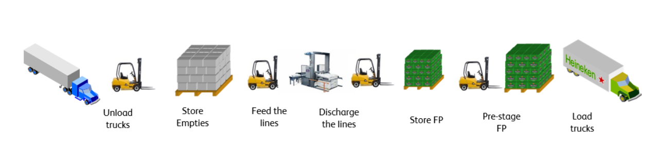
Figure 1: Example of internal flow in Heineken’s brewery. The process begins with “unload trucks,” where trucks with empties are discharged using forklifts. Next, “store empties” involves moving empties to the empty yard for storage. “Feed the lines” transfers empty bottles to production lines for filling. The “discharge the lines” step moves finished products (FP) to storage locations, followed by “pre-stage FP” to prepare orders for efficient truck loading. Finally, “load trucks” completes the process by loading FP into trucks for client delivery. Each step involves transportation and handling activities (Aussaresse 2023).

In determining the requirements of a facility, three important considerations are the flow systems, activity relationships, and space requirements. Flow depends on production and transfer lot sizes, unit load sizes, material handling systems, layout arrangement, and building configuration. Measuring flow involves the calculation of activity relationships between machines and departments. Space is a function of lot sizes, storage systems, production equipment type and size, layout arrangement, building configuration, housekeeping and organization policies, material handling equipment, office design, cafeteria design, and restroom design. As indicated in previous chapters, facilities planning is iterative. The planning team needs to interact with product, process, and schedule designers and with top management to identify issues and alternative strategies. Contemporary approaches such as decentralized storage, multiple receiving docks, deliveries to points of use, cellular manufacturing, lean structures, and small-lot purchasing and production can challenge traditional relationships and reduce flow and space requirements.

Some traditional relationships to challenge are centralized offices, a centralized storage area, a single receiving area, and a centralized rework area. Flow requirements are reduced with deliveries to points of use, decentralized storage close to points of use, pull strategies with kanbans, and manufacturing cells. Less space is then required for inventories; production, storage, and handling equipment; offices; parking lots; and cafeterias.

— Facilities Planning (Tompkins 2010, 83–84).

“Empties” are empty glass bottles ready to be filled on the production lines. “Unload trucks” is the first process step, in which trucks carrying empties are discharged with forklift trucks. “Store empties” brings them to the empty yard. “Feed the lines” brings empty bottles to production. “Discharge the lines” transfers finished products to storage. “Pre-stage FP” prepares orders so that trucks can be loaded efficiently. Finally, “load trucks” loads finished products for delivery to clients.

— Warehousing Trends and Innovations: Best Practices (Aussaresse 2023, 19).

Design steps

The design process encompasses the following steps, regardless of decision level (Rouwenhorst et al. 2000):

Data acquisition.
Functional and technical specifications.
Selection of means and equipment.
Layout planning.
Selection of planning and control policies.

Remember: facilities planning is an iterative process.

Warehouse design sequences

Design sequences vary, but follow similar steps.

Baker and Canessa (2009)

Define system requirements.
Define and obtain data.
Analyze data.
Establish the unit loads to use.
Determine operating procedures and methods.
Consider possible equipment types and characteristics.
Calculate equipment capacities and quantities.
Define services and ancillary operations.
Prepare possible layouts.
Evaluate and assess the alternatives.
Identify the preferred design.

Frazelle (2016)

Determine space requirements for all warehouse functions.
Locate functions with high adjacency requirements close to one another.
Assign high-storage activities to high-bay space and labor-intensive processes to low-bay space.
Determine flow paths.
Assign the optimal material-handling method to each flow path.
Minimize space requirements.
Develop and document expansion and contraction strategies.

The first six steps turn a business need into a defined operating concept. Requirements establish what the system must accomplish. Data collection and analysis quantify products, orders, arrivals, dispatches, costs, and the site. Unit-load and operating-method decisions then determine how goods will move and which equipment families are feasible. These choices are interdependent and may require iteration rather than one irreversible pass.

Oxley (1994) refers here to the overall system within which the warehouse operates, and therefore includes business strategy requirements and relevant constraints, such as planning and environmental issues. Approaches described in business and supply chain strategy literature, such as on competitive advantage and consumer value (Christopher, 2005) are relevant, as is the use of scenario planning (e.g. Sodhi, 2003). A framework to identify the role of warehousing within supply chains is given in Baker (2007a) and there are some checklists on warehouse roles (e.g. cross-docking) and functions (e.g. storage) within warehousing literature, for example in Higginson and Bookbinder (2005).

— Warehouse Design: A Structured Approach (Baker and Canessa 2009, 431, sec. 6.1).

Bodner et al. (2002) state the expert designer has a prespecified list of data to be requested, to which they may add depending on the precise nature of the project. The warehouse design companies surveyed support that checklists are often used by practitioners, normally formalised into database or spreadsheet models, ready for analysis. Flow charts may also be used to obtain information.

Such checklists of data are given in various publications, including Rowley (2000), McGinnis and Mulaik (2000), Bodner et al. (2002), Frazelle (2002b) and Rushton et al. (2006). These lists include product details, order profiles, goods arrival and despatch patterns, cost data and site information (where a site has already been identified).

— Warehouse Design: A Structured Approach (Baker and Canessa 2009, 431, sec. 6.2).

Database and spreadsheet models are normally used by practitioners to analyse data. Govindaraj et al. (2000) state that this process normally involves an analyst computing a number of routine statistics from the order database and then the designer uses his experience to interpret these statistics.

— Warehouse Design: A Structured Approach (Baker and Canessa 2009, 432, sec. 6.3).

Unit-load selection must account for supplier and customer implications across the supply chain.

There are few tools listed in the literature for this step, although Roll et al. (1989) do describe a systematic approach that develops a mathematical relationship between container size and storage cost and then proceed to describe a simulation approach that can be used where average values are not appropriate. Rushton et al. (2000) go on to explain that the choice of unit load cannot be taken in isolation but must take into account the whole supply chain (i.e. supplier and customer considerations).

It is evident from the responses that there is considerable reliance placed on the expertise of the individual warehouse designers. For example, one respondent stated that unit loads were established by “design experience and expertise, combined with iterative discussions with the client”.

— Warehouse Design: A Structured Approach (Baker and Canessa 2009, 433, sec. 6.4).

Operating procedures define the high-level method and zoning.

These are the high-level procedures and methods for each function of the warehouse. A wide variety of techniques are used by the respondents, including checklists, warehouse zoning, technology assessment charts, concept library, and standard work procedures.

An important part of this step is the decision as to the zones into which the warehouse should be divided (e.g. zones for different product groups, temperature regimes, or Pareto classifications). Again, this appears to be left to the experience of the warehouse designer. Based on the adopted zones, Rushton et al. (2006) describe warehouse flow diagrams that represent the daily flows passing through the various zones of a warehouse as a basis for the subsequent steps.

— Warehouse Design: A Structured Approach (Baker and Canessa 2009, 433, sec. 6.5).

Equipment screening may use heuristic, analytic, or simulation methods. Step 6 therefore hands a feasible equipment set to the capacity, layout, and evaluation work on the next slide.

In contrast to some of the previous steps, there are many tools available in the literature that may assist with the evaluation of equipment types. This is also reflected in the wide range of techniques used by the warehouse design companies, such as decision trees, matrices, SCOR assessments and factor analysis.

Ashayeri and Gelders (1985) identify three generic methods that assist chiefly, although not solely, with this step:

Heuristic methods (which are based on a close examination of different design alternatives through intuitive rules, based on experience);

Analytic methods (which are used to calculate an optimum solution);

Simulation methods (which conduct “what if” analyses).

— Warehouse Design: A Structured Approach (Baker and Canessa 2009, 433, sec. 6.6).

Step 7 converts the feasible equipment types from the previous slide into capacities and quantities. Step 8 adds services and ancillary requirements, which practitioners sometimes formalize with checklists. Step 9 turns these requirements into alternative layouts. Step 10 tests feasibility, requirement fit, and cost. Step 11 integrates the preferred unit loads, processes, systems, equipment, staffing, layouts, and costs into one coherent design.

This is generally a matter of calculation and formal spreadsheet models tend to be used, based on warehouse flows (as per Rushton et al., 2006) and performance standards (e.g. from historic KPIs or rated activity sampling). Many of the analytic and simulation methods, mentioned in the previous step, in fact address equipment capacities and quantities as well as the wider equipment selection question.

— Warehouse Design: A Structured Approach (Baker and Canessa 2009, 434, sec. 6.7).

The source explicitly limits what is known for step 8. It reports a practice-based checklist rather than a validated general methodology.

There are no real methodologies described in the literature for this step. It appears to be derived from the experience of the warehouse designers, sometimes formalised into checklists of requirements.

— Warehouse Design: A Structured Approach (Baker and Canessa 2009, 434, sec. 6.8).

All of the respondents use computer-aided design (CAD) software to assist in drawing up the layouts. Canen and Williamson (1996) provide a review the literature on computer-based layout packages and conclude that there is considerable software available. However, their research concluded that specialist warehouse layout software appeared to be little used by companies, who tend instead to use non-specialist software, such as AutoCAD. Such software tends to be an aid for an experienced designer to help draw the layout, as exemplified by one respondent who stated that layouts are prepared “by experience and use of AutoCAD to draft layouts”.

— Warehouse Design: A Structured Approach (Baker and Canessa 2009, 434, sec. 6.9).

Oxley (1994) states that this step is largely concerned with validating the operational and technical feasibility of the proposed solutions, checking that it meets the requirements of step one (i.e. the initial requirements), and undertaking capital and operational cost evaluations.

— Warehouse Design: A Structured Approach (Baker and Canessa 2009, 434, sec. 6.10).

This step is basically the drawing together of all of the above elements into a coherent design, identifying, for example, the unit loads to be used, the operations and flows, the information systems, the equipment types and quantities, the internal and external layouts, the staffing requirements and the costs (Oxley, 1994). No specific process is described in the literature for this step, but the warehouse design companies gave some examples of both quantitative (e.g. financial business case) and qualitative (e.g. SWOT analysis) methods.

— Warehouse Design: A Structured Approach (Baker and Canessa 2009, 435, sec. 6.11).

Warehouse layout is much like puzzle piecing. The puzzle pieces are the warehouse activities of receiving, receiving staging, pallet storage and retrieval, case picking, piece picking, packing, order assembly, shipping staging, and so on. As with a puzzle, it is impossible to complete until all the individual pieces have been shaped and sized. The individual shaping and sizing of those individual pieces were completed in previous chapters, where we selected equipment and determined space requirements for each activity. Our seven-step RightPaths methodology for putting those activities together into an efficient warehouse layout is the subject of this chapter.

Determine space requirements for all warehouse functions.

Locate functions with high adjacency requirements close to one another.

Assign activities with high storage requirements to high-bay space and labor-intensive processes in low-bay space.

Determine flow paths.

Assign the optimal material-handling method to each flow path.

Minimize space requirements.

Develop and document expansion/contraction strategies.

Warehouse layouts should be based primarily on the space requirements for and the interrelationships between warehouse activities. The first step in laying out a warehouse is to determine the overall space requirements for all warehouse activities. The Space Requirements Optimization from our RightHouse Layout Optimization System optimizes and summarizes long-term space requirements.

— World-Class Warehousing and Material Handling (Frazelle 2016, 291–92 (PDF pp. 307–308)).

Warehouse floor-space requirement planning

The main floor-space areas within the warehouse that need to be calculated are (Richards 2014):

Receiving area
Quarantine and inspection area
Reserve storage area
Carton-picking area
Item-pick area
Value-adding services area
Packing area

Dispatch area
Cross-dock area
Empty pallet and packaging storage area
MHE charging areas
Warehouse offices
Restrooms

The information collected to calculate space is normally current or historical. Future volumes and changes also need to be considered!

Floor-space planning begins with the complete activity system, not storage alone. Receiving, quarantine, reserve storage, picking, value-added work, packing, dispatch, cross-docking, support storage, charging, offices, and restrooms all compete for the same building envelope. The current profile is a starting point; future volumes, product changes, and peaks determine the design horizon.

The main floor-space areas within the warehouse that need to be calculated are as follows: receiving area; quarantine and inspection area; reserve storage area; carton-picking area; item-pick area; value-adding services area; packing area; despatch area; cross-dock area; empty pallet and packaging storage area; MHE charging areas; warehouse offices; and restrooms.

The information collected is normally current or historical and therefore future volumes and changes in product characteristics also need to be taken into account. Furthermore, the use of averages can be misleading, and you need to decide on how you deal with peaks in the business.

— Warehouse Management (Richards 2014, 205–7, sec. “Data collection and analysis”).

The figure shown in the notes is Frazelle’s Figure 9.1, not Richards’s figure. It represents the long-term space requirement for all warehouse activities.

Figure 2: Projected long-term overall space requirements for all warehouse activities (Frazelle 2016, 292–93, Figure 9.1).

Warehouse layouts should be based primarily on the space requirements for and the interrelationships between warehouse activities. The first step in laying out a warehouse is to determine the overall space requirements for all warehouse activities. The Space Requirements Optimization from our RightHouse Layout Optimization System optimizes and summarizes long-term space requirements (Figure 9.1).

— World-Class Warehousing and Material Handling (Frazelle 2016, 291–93, Figure 9.1).

Storage capacity requirements

Should we design storage to accommodate peaks in business, average activity, or somewhere in between?

Short-lived high peak-to-average storage ratio

Outside warehousing and/or trailer storage should be considered to accommodate the peak storage requirement if:

the duration of the peak is short-lived (<0.5 year), and
the peak-to-average storage ratio is high (> 1:5), then

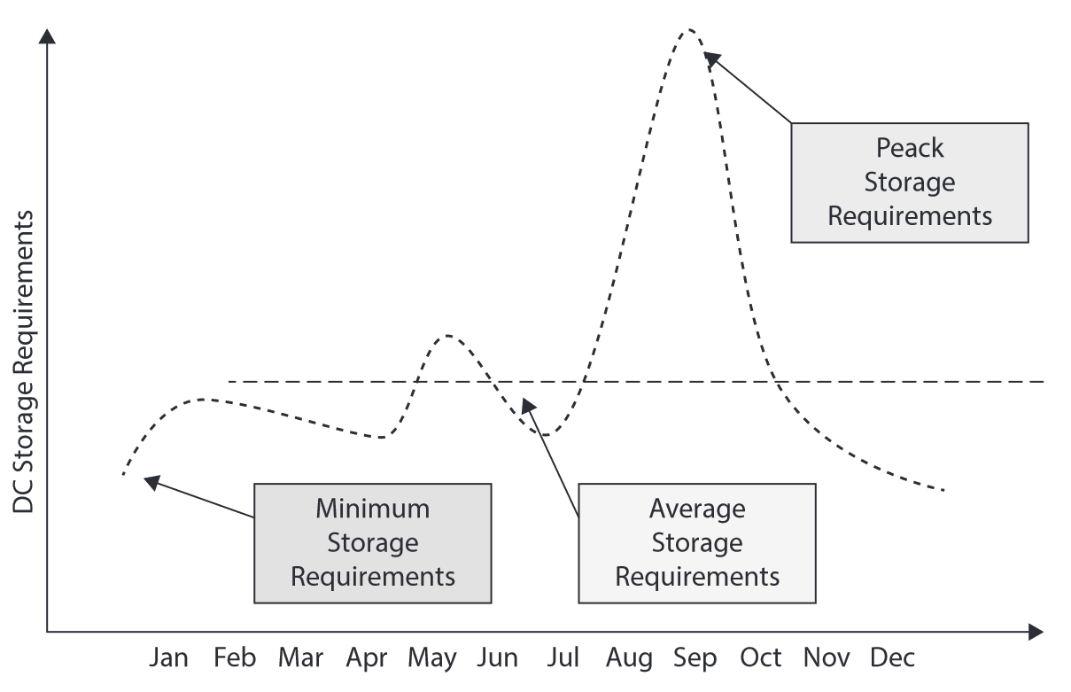
Figure 3: Storage capacity requirements with a short-lived high peak-to-average storage ratio (Frazelle 2016)

The decision concerns how much peak capacity to build permanently. When a large peak lasts for less than half a year, external warehousing or trailer storage can absorb the temporary excess. This avoids paying year-round for a building sized to a brief extreme. The source presents this as a planning consideration, not a rule that temporary space is automatically cheaper in every setting.

One of the most difficult decisions to make in storage-space planning is the portion of the peak storage requirements to accommodate. If the duration of the peak is short-lived and the peak-to-average storage ratio is high, then outside warehousing and/or trailer storage should be considered to accommodate the peak storage requirements (Figure 9.2).

— World-Class Warehousing and Material Handling (Frazelle 2016, 292–94, Figure 9.2).

Richards states the numerical planning threshold that the slide expresses as > 1:5 and <0.5 year.

Very few operations have a level volume of storage and activity throughout the year. For many companies there are a number of peaks and troughs. The question is whether we plan for and accommodate peaks in business, whether we design for the average activity or somewhere in between. According to Frazelle (2002), if the duration of the peak period is short and the ratio of peak to average is high, then it is worth considering temporary storage and labour for this overspill. If the peaks are extended and the ratio of peak to average is much smaller, the warehouse and labour requirements should be sized at or near peak requirements. The suggestion is that you size near to average if the ratio is more than 1:5 and the peak lasts for less than half a year. You should size near the peak when the ratio is less than 1:2 and the peaks last longer.

— Warehouse Management (Richards 2014, 206–7, sec. “Data collection and analysis”).

Low peak-to-average storage ratio

The storage area should be sized at or very near peak requirements if

the duration of the peak is for an extended period and
the peak-to-average storage ratio is low (< 1:2).

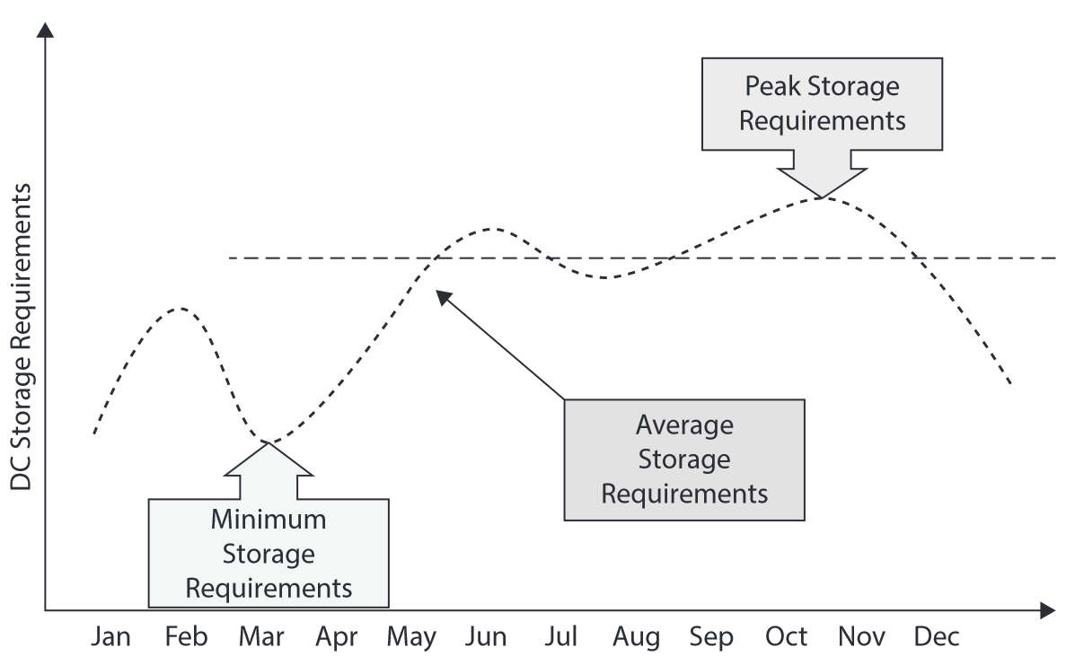
Figure 4: Storage capacity requirements over time with a low peak-to-average storage ratio (Frazelle 2016)

Here the peak is sustained rather than exceptional. When demand remains near the peak for an extended period, temporary overflow would become a recurring operating condition. Sizing storage near the peak therefore provides permanent capacity for the level the operation regularly experiences. The ratio convention below is preserved exactly as the slide states it.

If the duration of the peak is for an extended period and the peak-to-average storage ratio is low, then the storage area should be sized at or very near peak requirements (Figure 9.3).

— World-Class Warehousing and Material Handling (Frazelle 2016, 292–94, Figure 9.3).

Richards states the numerical planning threshold that the slide expresses as < 1:2.

Very few operations have a level volume of storage and activity throughout the year. For many companies there are a number of peaks and troughs. The question is whether we plan for and accommodate peaks in business, whether we design for the average activity or somewhere in between. According to Frazelle (2002), if the duration of the peak period is short and the ratio of peak to average is high, then it is worth considering temporary storage and labour for this overspill. If the peaks are extended and the ratio of peak to average is much smaller, the warehouse and labour requirements should be sized at or near peak requirements. The suggestion is that you size near to average if the ratio is more than 1:5 and the peak lasts for less than half a year. You should size near the peak when the ratio is less than 1:2 and the peaks last longer.

— Warehouse Management (Richards 2014, 206–7, sec. “Data collection and analysis”).

Occupancy vs. productivity

For storage planning purposes, we assume only a portion of the warehouse locations will be occupied.

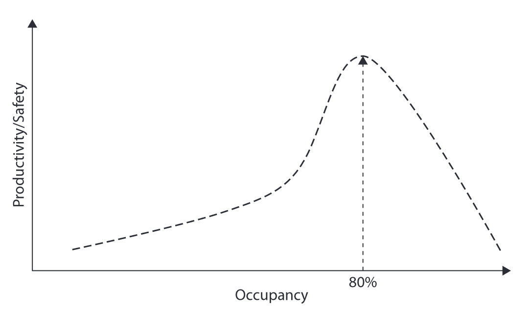
Figure 5: As the utilization of storage locations exceeds 85% in non-real-time warehouses and 90% in real-time warehouses, the productivity and safety of the operations decline dramatically (Frazelle 2016)

Planning for less than 100% occupancy preserves choice. Put-away can select a safe, suitable location without first moving other stock, and replenishment and retrieval retain enough maneuvering room. At very high occupancy, the time spent searching for space and rearranging inventory rises. Frazelle’s 85% and 90% figures are source-specific planning thresholds, not universal regulatory limits.

Another important consideration in storage space requirements planning is the portion of warehouse locations that will be occupied for planning purposes. As the utilization of storage locations exceeds 85 percent in non-real-time warehouses and 90 percent in real-time warehouses, the productivity and safety of the operations decline dramatically (Figure 9.4).

— World-Class Warehousing and Material Handling (Frazelle 2016, 294–95, Figure 9.4).

Storage total floor space

Calculating the total floor space depends on several factors, such as product, demand, MHE, and building characteristics.

Figure 6: Number of pallet locations required and the **height requirement** for each location (based on Richards 2014)

Figure 7: SKU characteristics and **possible storage media** (based on Richards 2014)

Calculating the amount of storage space required and the storage medium depends on a large number of factors. Each item needs to be evaluated and a table produced to record the different item properties and as a result decide on potential storage media. Having calculated the amount of items stored per product line and converted these into pallet quantities, we are able to calculate the total number of pallets we need to store, by product line. Once this has been calculated, produce a chart detailing the number of pallet locations required and the height requirement for each location (Table 9.1). Depending on the nature of the product in terms of weight, crushability, etc, it is likely that the pallet heights will vary between products and some products may only require bin or tote storage as the quantities are so low. The next decision is the type of storage medium to use. This can include block stacking, pallet racking, automated storage, shelf and bin locations or a combination of some or all. Table 9.2 shows the characteristics of each individual stock item and the possible storage media envisaged. As can be seen from Table 9.2, we have recorded as much information as possible regarding the storage and order profile of the products listed. This gives us the opportunity to decide on the most suitable storage and handling medium. A similar table can be produced to determine the size of the pick face location(s) for each product where we need to take into account the average and maximum amount of product despatched per day. The idea is to make sure that we do not have to replenish these locations during picking and therefore we need to size the locations appropriately based on the number of items picked per day. The number and size of the pick locations will depend on the available ground floor locations (initially) and cubic capacity of those locations. Having produced a rule-of-thumb formula for calculating dock space there is a formula to calculate the number of pallets that can be stored within a given cubic area when using standard adjustable pallet racking. This is as follows: (Number of width modules × pallets in a module width) × (number of length modules × pallets in module length) × number of height modules where: Module width = width of aisle + 2 pallet lengths (short side) + clearance between back-to-back pallets Module length = width of upright + 3 × clearance + 2 pallets (long side) Module height = height of pallet + clearance above pallet plus racking beam height

— Warehouse Management: A Complete Guide to Improving Efficiency and Minimizing Costs in the Modern Warehouse (Richards 2014, 208–13).

Storage density: equipment and space

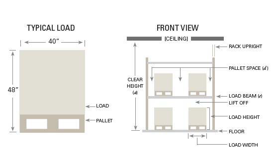
Figure 8: Storage equipment and pallet space requirements.

The diagram is cropped from The Raymond Corporation’s official Storage Space Efficiency Guide: A Demonstration in Space, p. 14, “Calculating the Cube for Pallet Storage” (The Raymond Corporation 2018). The crop retains the source’s US customary dimensions. Use the geometry to understand how pallet size, rack uprights, beam height, lift-off clearance, load height, clear height, and aisle width combine; do not transfer those numerical dimensions to a metric design. The source’s worked space example also excludes intersecting aisles, columns, and dock space.

To calculate the storage space required per pallet, you can apply the formula shown below.

— Storage Space Efficiency Guide: A Demonstration in Space (The Raymond Corporation 2018, 14, sec. “Calculating the Cube for Pallet Storage”).

Richards explains why a pallet-space diagram is only a starting point:

The number of pallets that can be stored in this particular area is determined, in the main, by the aisle width, type of racking and the size of pallet. As mentioned earlier, this is a rule-of-thumb calculation and other factors need to be taken into account before committing to these figures. The calculations take into account the aisles between the racking but do not take into account aisles and gangways at the front of the racking. They do not take into account potential pallet overhang, rear walkways and fire exits.

— Warehouse Management (Richards 2014, 212–14, secs. “Other factors” and “Aisle width”).

Deciding on the optimal aisle width is a critical part of an overall storage/ materials-handling strategy. Aisle width decisions need to achieve the best combination of productivity, space utilization, flexibility, safety and equipment costs for the specific application (Piasecki 2002). Other factors include the depth of the pallet on the truck and whether there is a requirement for two trucks to pass in the aisle.

— Warehouse Management (Richards 2014, 214, sec. “Aisle width”).

Storage density: pallet footprint

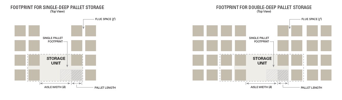
Figure 9: Pallet footprint in single- and double-deep storage.

Floor space calculations use a storage density factor that varies by storage medium and MHE.

Factors influencing space planning

Other factors that need to be taken into account are: - Planned utilization within the warehouse. It is agreed that once storage utilization exceeds 85 per cent, productivity and safety decline. The operation will slow appreciably as put-away is delayed whilst space is being freed up. - The presence and location of roof columns. Storage equipment manufacturers will take this into account when producing plans. - The requirement for space between the backs of pallets (flue) and at the sides of pallets. - The presence and location of sprinklers (ceiling or in rack). The overhead pipes and sprinklers will limit the height both within the warehouse and within the racking itself. - The type of lighting utilized and any heating or cooling systems installed. - Lift height of forklift truck. Different types of forklift truck will have different lift-height capabilities. Pallet orientation (short facing or long facing). How a pallet is stored within the racking has its own trade-off within the warehouse. Storing a pallet with the long face parallel to the aisle makes it easier for operators to pick, not having to stretch too far across the pallet. However, storing the pallet with the short side parallel to the aisle means greater flexibility (UK and euro pallets can be stored in the same bay) and more pallets can be stored in a length of racking. Number of pallets per beam (three pallets between the uprights will increase the number of pallets stored by removing a number of uprights). This can save up to 4 per cent of space. However, the maximum weight per beam needs to be adhered to. - The requirement for cross aisles within the racking to reduce travel and the need for walkways between the end of the racking and the wall to provide escape routes for staff. - Type of racking, for example: – Double-deep racking will reduce the number of aisles required. – Narrow aisle storage requires less aisle width. – Drive-in or satellite racking doesn’t operate with aisles. – Flow racks only require two aisles depending on the length of the lane or potentially three if they are operated back to back. If the operation is planning to have pick faces on the floor, ie underneath the reserve storage racks, we need to take into account the total number of floor locations that will be set aside for carton-pick locations and shelf locations. We also need to be aware of part-pallet receipts and part-pallet locations if we have to pick from height.

— Warehouse Management: A Complete Guide to Improving Efficiency and Minimizing Costs in the Modern Warehouse (Richards 2014, 212–13).

Calculation steps

Calculate the average unit inventory as a function of the annual demand and inventory turn rate¹:

\[ \text{Avg. unit inventory} = \frac{\text{Forecasted unit sales}}{\text{Annual inventory turns}} \]

Then, calculate the average pallet inventory:

\[ \text{Avg. pallet inventory} = \frac{\text{Avg. unit inventory}}{\text{Avg. units/pallet}} \]

Next, calculate the peak (pallet) inventory:

\[ \text{Peak inventory} = \text{Avg. inventory}\times\text{Peak-to-average ratio} \]

Only a portion of peak inventory is considered to compute the storage capacity:

\[ \begin{aligned} \text{Effective storage capacity} &= \text{Pct. peak planning} \\ &\quad \times \text{Peak inventory} \end{aligned} \]

The required number of pallet positions is divided by a location utilization factor²:

\[ \text{Inventory positions} = \frac{\text{Effective storage capacity}}{\text{Location utilization factor}} \]

Floor space requirements are calculated using a predetermined storage density:

\[ \text{Floor space} = \text{Inventory positions}\times\text{Storage density} \]

Stihl Corporation recently asked us to assist them in projecting their long-term warehouse space requirements. Because pallet storage occupies the most space, we began by computing the storage-space requirements for pallets. The computations and scenarios are described next and illustrated in Figure 9.5.

Divide forecasted unit sales by annual inventory turns to compute the average unit inventory.

Divide the average unit inventory by the average units per pallet to compute the average pallet inventory.

Multiply the average pallet inventory by the ratio of peak-to-average inventory to compute the peak pallet inventory.

Multiply the peak pallet inventory by the portion of peak inventory used for storage planning purposes to compute the effective pallet storage capacity.

Divide the effective pallet storage capacity by the location utilization factor (typically 85 percent for single-deep pallet storage) to compute the required number of pallet storage locations.

Multiply the required number of pallet storage locations by the storage density (square feet per pallet computed as a function of the aisle width and storage height) to compute the floor-space requirements.

Apply the annual occupancy cost rate to estimate the annual occupancy costs.

— World-Class Warehousing and Material Handling [Frazelle (2016), pp. 294–297 (PDF pp. 310–313; annotation p. 312)].

Finding additional space

When facing a shortage of space, warehouse managers could consider:

Expanding the warehouse
Renting additional space
Creating more space within the existing premises
- Reducing inventory levels (e.g., excluding slow movers)
- Changing storage and MHE
- Consolidating stock (trade-off with labor)
- Reducing beam heights (accommodate half-, quarter-pallets)
- Moving from fixed locations to random locations.
- Using temporary storage structures (e.g., sea containers and trailers)

When facing a shortage of space within the warehouse there are a number of options available, namely: - expanding the warehouse; - renting additional space; and - creating more space within the existing premises. If the company is unwilling or cannot afford to rent external space and is unable to expand the existing warehouse or make significant structural changes there are ways of increasing the number of storage locations without major upheavals. A potential solution to increasing available space within a warehouse is to reduce inventory levels. Unfortunately, this tends to be beyond the remit of the warehouse manager. However, warehouse managers can identify slow and non-moving stock with a view to disposing of it in agreement with the sales and finance departments. Although it may sound strange to suggest looking within the existing facility, there are options that might have been overlooked. Some potential options are as follows: - Change the type of storage medium or mechanical handling equipment used. This can include changing from single-deep to double-deep racks, utilizing drive-in racking, narrow aisle racking or introducing articulated forklift trucks which can operate in narrower aisles. - Consolidation of stock. Unless stock items have different best-before codes, batch numbers or expiry dates it is worth checking how many part pallets there are of certain items and spending time consolidating them. This does require the use of labour but the trade-off is between the freeing up of additional space and this cost. The alternative is renting space at a third-party warehouse. Some warehouse systems allow the storage of different products in the same location. This will require careful planning and additional training. - Reducing beam heights within the warehouse to accommodate smaller, full or part pallets. How many times have you entered a warehouse to see half metre high pallets in 2 metre high locations, not including pick locations, of course? Many warehouses prefer to have standard-height pallet locations as it is easier to manage and control and is more pleasing on the eye. However, the potential for optimum space utilization is lost. - As the majority of warehouses operate with adjustable pallet racking the most cost-effective method of storage is to have variable height locations. These will accommodate 0.5 metre, 1 metre, 1.2 metre, 1.5 metre and 2 metre pallet heights, for example. - Moving from fixed locations to random locations. In a warehouse with fixed locations the same product is always held in the same location, irrespective of quantity. With fixed locations if an item is out of stock you cannot use that location for anything else. - If there is sufficient space in the yard a temporary storage structure may be the answer or the use of sea containers or trailers. Security and the potential for water damage are areas that need to be considered before embarking on such a solution.

— Warehouse Management: A Complete Guide to Improving Efficiency and Minimizing Costs in the Modern Warehouse (Richards 2014, 217–18).

Activity relationships

Helps evaluate alternative department-layout arrangements.

Quantitative measures

Used in facilities having large volumes of materials, information, and people moving between departments.
Examples:
- pieces per hour
- moves per day
- kg per week

Qualitative measures

Used in facilities having significant communication and organizational interrelations.
Ranges from
1. absolute necessity that two departments be close to each other
2. preference that two departments not be close to each other

Frequently, a facility will have a need for both quantitative and qualitative measures of flow.

ACTIVITY RELATIONSHIPS

Measuring the activities among departments is one of the most important elements in the layout of departments within a facility. To evaluate alternative arrangements, activity relationships must be established. Activity relationships may be specified in a quantitative or qualitative manner. Quantitative measures may include pieces per hour, moves per day, or pounds per week. Qualitative measures may range from an absolute necessity that two departments be close to each other to a preference that two departments not be close to each other. In facilities having large volumes of materials, information, and people moving between departments, a quantitative measure of flow will typically be the basis for the arrangement of departments. On the contrary, in facilities having very little actual movement of materials, information, and people flowing between departments, but having significant communication and organizational interrelations, a qualitative measure of flow will typically serve as the basis for the arrangement of departments. Most often, a facility will have a need for both quantitative and qualitative measures of flow, and both measures should be used. A chart that can be useful in flow measurement is the mileage chart shown in Figure 3.38. Notice that the diagonal of the mileage chart is blank, since the question “How far is it from New York to New York?” makes little sense. Furthermore, the mileage chart is a symmetric matrix. (Distance charts do not have to be symmetric; if one-way aisles or roads are used, distance between two points will seldom be symmetric.) In Figure 3.38, it is 963 miles from Boston to Chicago and also 963 miles from Chicago to Boston. When distances between two cities are symmetric, the mileage can be represented in a triangular mileage chart as shown in Figure 3.39. The distance matrix is not symmetric when the routes are not bidirectional, as in the case of one-way streets. The mileage chart will also vary depending on the driving objective. A scenic route typically involves longer distance. Additionally, the method of transport will impact the distance traveled. Travel by commercial airlines will be shorter in both distance and time.

— Facilities Planning (Tompkins 2010, 113–14 (PDF p. 125)).

Quantitative flow measurement

Measurements recorded in a from-to-chart in terms of the amount moved between departments.
To create a from-to-chart:
1. List all departments down the row and across the column following the overall flow pattern.
2. Establish a measure of flow for the facility that accurately indicates equivalent flow volumes.
3. If the items moved are equivalent regarding ease of movement, the number of trips may be recorded in the from-to chart.
4. If the items moved vary in size, weight, value, risk of damage, shape, and so on, then some common unit of measure may be established so that the quantities recorded in the from-to chart represent the proper relationships among the volumes of movement.
5. Based on the flow paths for the items to be moved and the established measure of flow, record the flow volumes in the from-to chart.

Flows may be measured quantitatively in terms of the amount moved between departments. The chart most often used to record these flows is a from-to chart. As can be seen in Figure 3.40, a from-to chart resembles the mileage chart given in Figure 3.38. The from-to chart is a square matrix but is seldom symmetric. The lack of symmetry is because there is no definite reason for the flows from stores to milling to be the same as the flows from milling to stores. A from-to chart is constructed as follows: 1. List all departments down the row and across the column following the overall flow pattern. For example, Figure 3.32 shows various flow patterns that can result in the departments listed in Figure 3.41. 2. Establish a measure of flow for the facility that accurately indicates equivalent flow volumes. If the items moved are equivalent with respect to ease of movement, the number of trips may be recorded in the from-to chart. If the items moved vary in size, weight, value, risk of damage, shape, and so on, then some common unit of measure may be established so that the quantities recorded in the from-to chart represent the proper relationships among the volumes of movement. 3. Based on the flow paths for the items to be moved and the established measure of flow, record the flow volumes in the from-to chart.

— Facilities Planning (Tompkins 2010, 114–16 (PDF p. 128)).

Example: developing the from-to chart

1/3 · Equivalent flow and routing. Use a common movement unit before adding flows (Tompkins 2010).

Assumed linear layout (overall flow →): A → C → B → D → E.

Component	Units/day	Movement factor	Equivalent flow/day	Routing
1	30	1	30 × 1 = 30	A → C → B → D → E
2	12	1	12 × 1 = 12	A → B → D → E
3	7	2	7 × 2 = 14	A → C → D → B → E

Each consecutive pair is a directed move.

Component 3 contributes 14, rather than 7, to A → C, C → D, D → B, and B → E.

The movement factor converts unlike components into a common flow unit. Components 1 and 2 each count as one equivalent move; component 3 counts as two because it is almost twice as large. For every component, place its equivalent daily flow on each consecutive routing leg. With departments ordered A-C-B-D-E, entries below the main diagonal identify backtracking against that overall direction. Entries near the diagonal represent shorter moves in this linear ordering.

A firm produces three components. Components 1 and 2 have the same size and weight and are equivalent with respect to movement. Component 3 is almost twice as large, and moving two units of either component 1 or 2 is equivalent to moving 1 unit of component 3. Thus, a movement factor of 2 is assigned to component 3. The departments included in the facility are A, B, C, D, and E. For this illustration, we assume that the departments are arranged in a linear flow pattern in the order A-C-B-D-E. The quantities to be produced and the component routings are as follows:

Component Production quantity per day Movement factor Equivalent flow per day Routing

1 30 1 30 A-C-B-D-E

2 12 1 12 A-B-D-E

3 7 2 14 A-C-D-B-E

The first step in creating the from-to chart is to list the departments in order of the overall flow down the rows and across the columns. Then, by considering each unit of component 3 moved to be equivalent to two moves of components 1 and 2, the flow volumes may be recorded as shown in Figure 3.42. Notice that flow volumes below the diagonal represent backtracking, and the closer the flow volumes are to the main diagonal, the shorter will be the move in the facility.

— Facilities Planning (Tompkins 2010, 116–17 (PDF pp. 128–129)).

Example: developing the from-to chart

2/3 · Build the chart. Assumed linear layout: A → C → B → D → E (overall flow →).

Component 1 · 30/day

A → C → B → D → E

Add 30 to A–C, C–B, B–D, and D–E.

Component 2 · 12/day

A → B → D → E

Add 12 to A–B, B–D, and D–E.

Component 3 · 14/day

A → C → D → B → E

Add 14 to A–C, C–D, D–B, and B–E.

From ↓ / To → · Equivalent flow/day

	A	C	B	D	E
A	—	30+ 14 44	12 12	0	0
C	0	—	30 30	14 14	0
B	0	0	—	30+ 12 42	14 14
D	0	0	14 14	—	30+ 12 42
E	0	0	0	0	—

A → C = 30 + 14 = 44. Sum contributions within each cell.

D → B = 14: returns to an earlier department in this layout (backtracking).

Linear layout, component data, and routing: Tompkins (2010).

Use the next-slide key four times. The first three fragment groups add the equivalent flows of components 1, 2, and 3. The fourth group replaces the contributions with totals and reveals zero-flow cells. Moving backward restores the previous contributions. Add each component’s equivalent flow to every consecutive leg of its route. Tompkins explicitly assumes a physical linear layout in the order A-C-B-D-E. D-to-B returns from the fourth department to the third, against the overall flow direction. The chart’s rows and columns follow that physical order, so this entry lies below the main diagonal. For an arbitrary row/column order, being below the diagonal alone does not establish physical backtracking. No department spacing or travel distance is specified in this example.

For this illustration, we assume that the departments are arranged in a linear flow pattern in the order A-C-B-D-E.

The first step in creating the from-to chart is to list the departments in order of the overall flow down the rows and across the columns.

— Facilities Planning (Tompkins 2010, 116–17 (PDF pp. 128–129)).

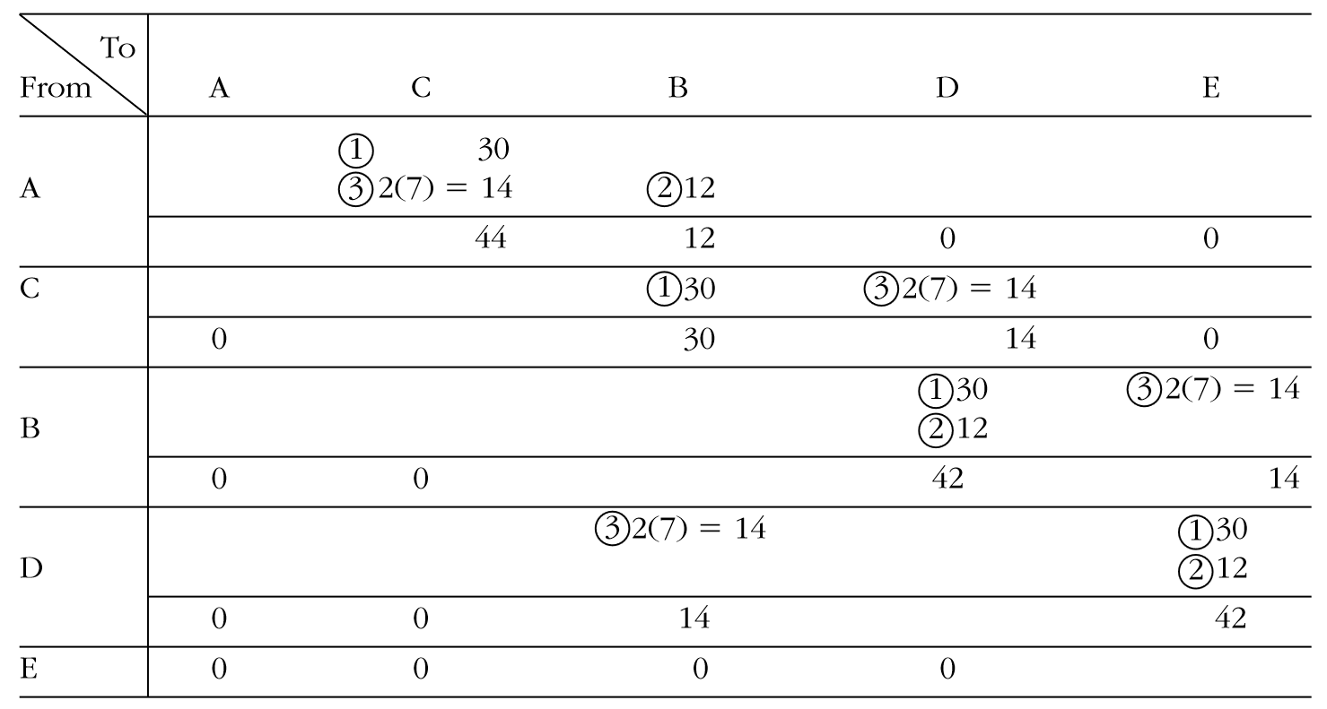
Example: developing the from-to chart

3/3 · Completed chart. Check the flows against the component routes.

Figure 10: 3 components being transported through departments A–E arranged in order A-C-B-D-E. Components 1 and 2 have the same size and weight, and component 3 is almost twice as large (thus movement factor is 2) (Tompkins 2010)

Figure 11: From-to chart indicates the volume of equivalent flows for each (circled) component (Tompkins 2010)

A firm produces three components. Components 1 and 2 have the same size and weight and are equivalent with respect to movement. Component 3 is almost twice as large, and moving two units of either component 1 or 2 is equivalent to moving 1 unit of component 3. Thus, a movement factor of 2 is assigned to component 3. The departments included in the facility are A, B, C, D, and E. For this illustration, we assume that the departments are arranged in a linear flow pattern in the order A-C-B-D-E. The quantities to be produced and the component routings are as follows:

Component Production quantity per day Movement factor Equivalent flow per day Routing

1 30 1 30 A-C-B-D-E

2 12 1 12 A-B-D-E

3 7 2 14 A-C-D-B-E

The first step in creating the from-to chart is to list the departments in order of the overall flow down the rows and across the columns. Then, by considering each unit of component 3 moved to be equivalent to two moves of components 1 and 2, the flow volumes may be recorded as shown in Figure 3.42. Notice that flow volumes below the diagonal represent backtracking, and the closer the flow volumes are to the main diagonal, the shorter will be the move in the facility.

— Facilities Planning (Tompkins 2010, 116–17 (PDF pp. 128–129)).

Qualitative flow measurement

Measures flow using the closeness relationship ratings developed by Muther and Hales (2015).
A relationship chart may be constructed as follows:
1. List all departments on the relationship chart.
2. Conduct interviews or surveys with persons from each department listed on the relationship chart and with the management responsible for all departments.
3. Define the criteria for assigning closeness relationships and itemize and record the criteria as the reasons for relationship values on the relationship chart.
4. Establish the relationship value and the reason for the value for all pairs of departments.
5. Allow everyone having input to the development of the relationship chart an opportunity to evaluate and discuss changes in the chart.

A relationship chart records every activity pair once, so the relationship is symmetric. Its upper half states the desired closeness; its lower half records coded reasons. The source sequence below explains the chart’s purpose, construction, scale, evidence, and reconciliation.

“The relationship chart is a cross-section form where the relationship between each activity1 (or function or area) and all other activities can be recorded. The basis of the form is shown in Figure 5-1.

The word “Activity” is a universal term, used throughout this book to designate “things” (other than people and process material) to be located as part of the layout planning. It encompasses, at different levels of planning or in different situations: department, area, function, work center, building, building feature, machine group, operation, and the like.

The relationship chart shows which activities have a relationship to others. Also, it rates the importance of the closeness between them and supports the rating with coded back-up reasons. These measures make the relationship chart one of the most highly practical and effective tools available for layout planning. It is undoubtedly the best way of integrating supporting services with the operating or producing departments and of planning the arrangement of office or service areas having little or no flow of materials.

The chart itself is almost self-explanatory. Where the activity on down-sloping line 1 intersects the activity represented by up-sloping line 3, the relationship between activity 1 and activity 3 is recorded. In this way, there is an intersecting ‘box’ for each pair of activities involved. The basic idea is how to show which activities should be located close together and which far apart, with all in-between relationships also rated relatively and recorded.

The chart can be likened to a from-to chart which has been folded diagonally so that the from-to and the to-from boxes fall on top of each other. The relationship chart thus shows the total relationship, i.e., in both directions.”

— Systematic Layout Planning (Muther and Hales 2015, chap. 5, pp. 5-2–5-3).

“Closeness is rated according to a value scale A, E, I, O, U, and X. A indicates closeness absolutely necessary; X indicates closeness is undesirable and the activities should be kept apart. E, I, O, and U each indicate varying degrees of closeness.

The closeness rating is more meaningful when reasons are tied to the rating. For each reason, a code number is assigned and an explanation is recorded in the ‘reason block’ on the sheet. That code number is then entered in its appropriate box(es). This way, two or three reasons can be marked in a relationship box without too much crowding. With this form, a great deal of information is gathered on one page without the need for lengthy notes.”

— Systematic Layout Planning (Muther and Hales 2015, chap. 5, p. 5-5).

A U rating means proximity is unimportant, whereas X means proximity is undesirable and the activities should be kept apart.

“3. Opinions can be solicited from others involved with the operation or its support in face-to-face discussion. This is frequently done at the same time information on which to base space requirements is gathered. When trying to get others to understand the relative degree of closeness which each vowel letter represents, the planner is wise to establish typical”benchmark relationships,” or benchmark ratings similar to those shown in Figure 5-6.

Questionnaires like the one in Figure 5-7 can be distributed to persons in charge of the activities involved. The planner cross-compares the responses and posts them on the relationship chart. But note that when two respondents differ in their ratings, the planner will have to follow-up with each to clarify and resolve their differences into a single, reason-supported rating. This reconciliation may take several days or longer.

The fastest, most effective way to complete the relationship chart is to assemble a small team to decide jointly on each relationship, the planner or one team member serving as recorder. In this way, hundreds of relationships can be captured in a few hours. For best results, the team should include one or more “voices” for each activity-area – typically supervisors and lead operators. (One way that helps the group keep in mind the specific pair of activities under consideration is to have a set of cards with the number and name of an activity printed clearly and boldly on each card and to have a pair of cards always on the discussion table.)”

— Systematic Layout Planning (Muther and Hales 2015, chap. 5, pp. 5-10–5-11).

Example of relationship chart

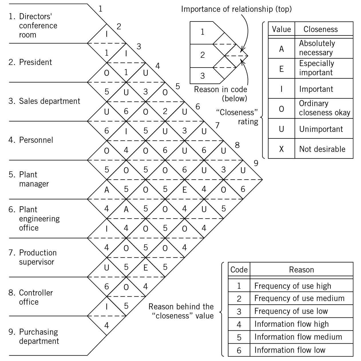
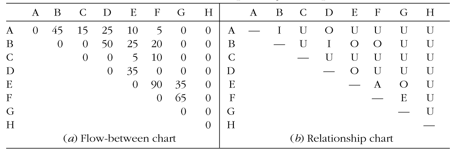
Figure 12: Example of closeness relationship chart (Tompkins 2010).

Flows may be measured qualitatively using closeness relationship values. The values may be recorded together with the reasons for each value in a relationship chart. Constructing the chart requires listing all departments, gathering input from the departments and management, defining the criteria for closeness relationships, establishing a value and reason for every department pair, and allowing all contributors to evaluate the result.

The facilities planner should synthesize the relationships because the chart requires the relationship value between departments A and B to equal the value between departments B and A. It is also important to distinguish U (unimportant) from X (undesirable). Departments with a U relationship may be adjacent and neither gain nor lose from proximity. Departments with an X relationship cannot be adjacent because of environmental, safety, or facilities constraints.

— Facilities Planning (Tompkins 2010, 117–19).

Warehouse activity relationship

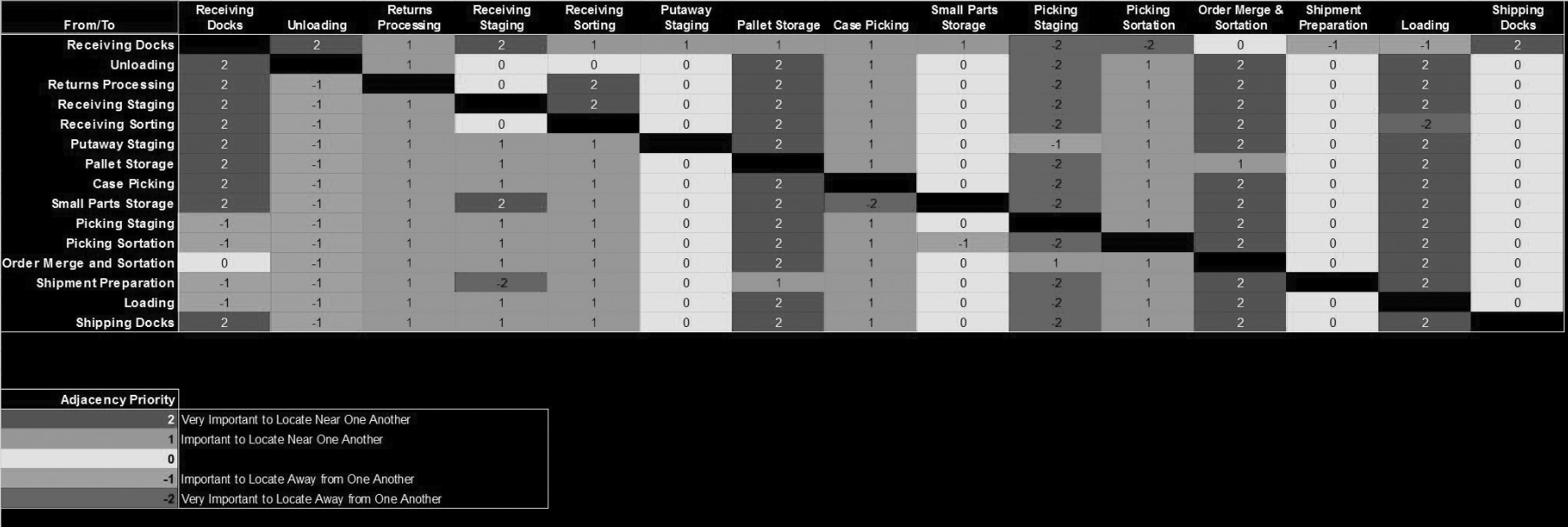
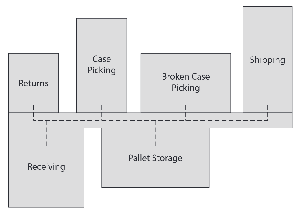
Figure 13: Importance of locating the processes adjacent to one another. For example, it is critical that reserve storage be adjacent to receiving staging for efficient put-away. (Frazelle 2016)

Systematic Layout Planning (SLP)

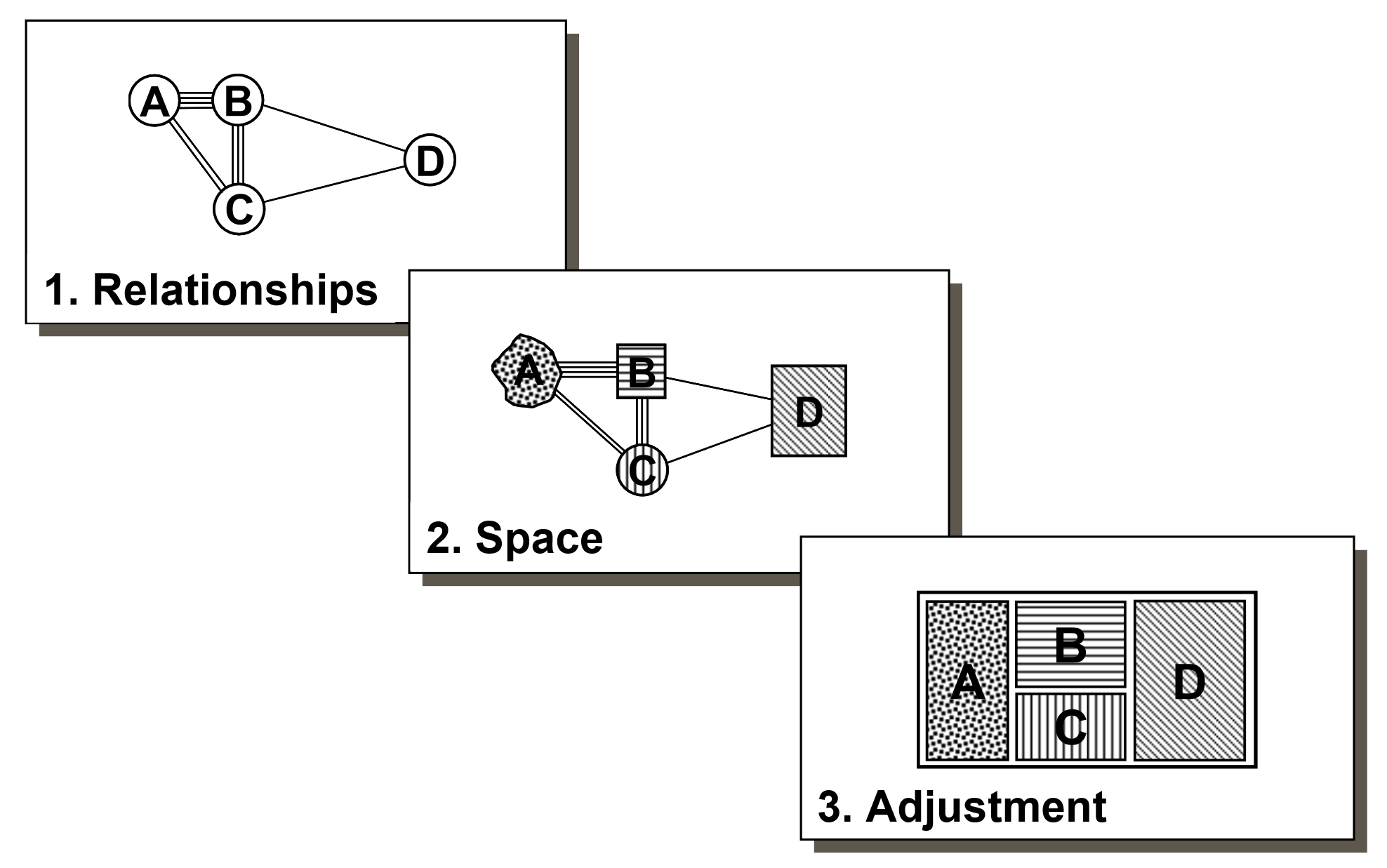
Figure 14: SLP activities: (1) establishing relationships between the layout activities, (2) determining space and dimensions required for each activity, and (3) adjusting relationships and space into an effective plan (see details on Richard Muther 2005; Muther and Hales 2015).

The figure on the slide presents the three SLP fundamentals as summarized in Muther’s 2005 overview (Richard Muther 2005, 2–3). The primary 2015 edition defines both the overall method and those three fundamentals.

“Systematic Layout Planning (SLP) consists of a framework of phases through which each layout project passes; a pattern of procedures for step-by-step planning; and a set of conventions for identifying, visualizing, and rating the various activities, relationships, and alternatives involved in any layout project.”

— Systematic Layout Planning (Muther and Hales 2015, preface, p. ix).

“Systematic Layout Planning is an organized way to conduct layout planning. It consists of a framework of phases, a pattern of procedures, and a set of conventions for identifying, rating, and visualizing the elements and areas involved in planning a layout.”

— Systematic Layout Planning (Muther and Hales 2015, chap. 2, p. 2-1).

“We explained the framework of four phases in Chapter 1. In this chapter, the Systematic Layout Planning pattern of procedures is described. The conventions will be introduced at the appropriate places in later chapters.

The strictly “layout planning” phases of any facilities rearrangement involve creating a general overall layout (Phase II) and, subsequently, a detailed layout plan (Phase III) for each portion of the general overall layout. In both Phase II and Phase III, the pattern to be followed is essentially the same.”

— Systematic Layout Planning (Muther and Hales 2015, chap. 2, p. 2-1).

“Every layout rests on the three fundamentals:

Relationships – the relative degree of closeness desired or required among things

Space – the amount, kind, and shape or configuration of the things being laid out

Adjustment – the arrangement of things into a realistic best fit

These three are always the heart of any layout planning project, regardless of products, processes, or size of project. It is therefore logical and to be expected that the pattern of layout planning procedures is based directly on these fundamentals. See Figure 2-1.”

— Systematic Layout Planning (Muther and Hales 2015, chap. 2, pp. 2-1–2-2).

From-to-chart to relationship score

Convert the from-to chart into a relationship score using closeness ratings:
1. Aggregate flows \(f_{ij}\) and \(f_{ji}\) to create a symmetric flow-between chart.
2. Divide the maximum flow value into intervals. For example, ratings A, E, I, O, and U lead to five intervals.
3. Assign a closeness rating to each pair of departments based on the interval in which the flow value falls.

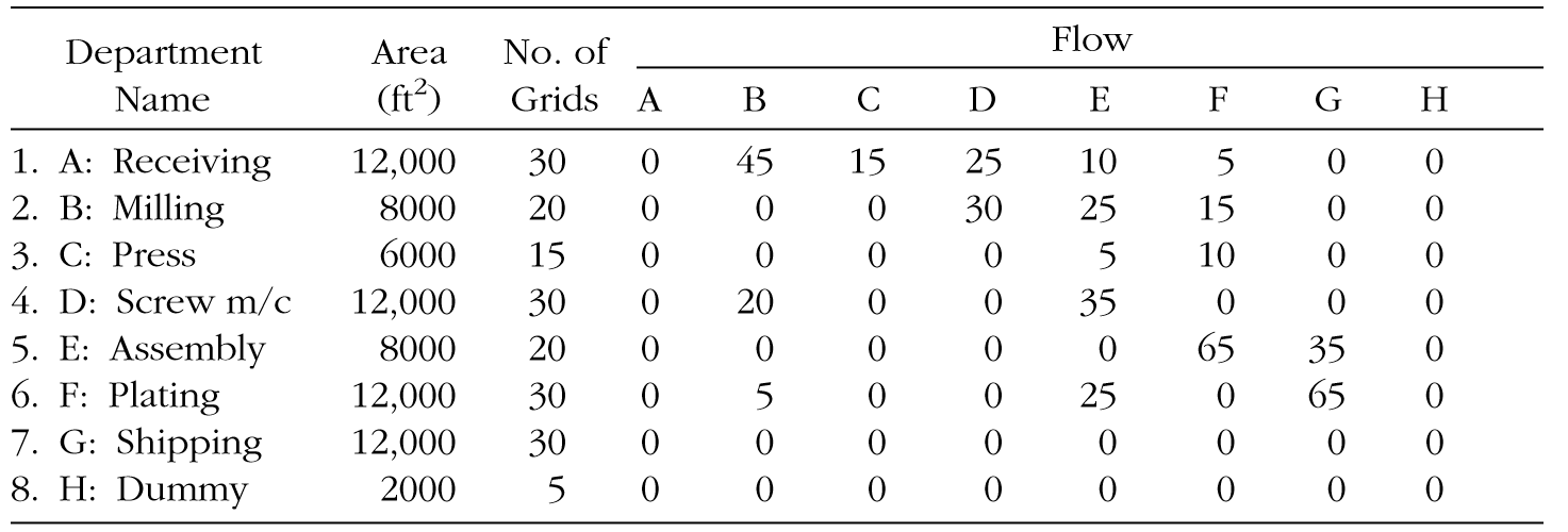
Figure 15: Departmental data and from-to chart. (Tompkins 2010)

No. of grids = number of equal-area layout cells assigned to a department.

Here, one 20 ft × 20 ft cell = 400 ft² (≈ 37.16 m²). Receiving: 12,000 / 400 = 30 cells.

Figure 16: Flows \(f_{ij}\) and \(f_{ji}\) are added to create a symmetric flow-between chart. Then, the maximum value of the flow-between chart (i.e., 90) is divided into five 18-units intervals (viz., A=73–90, E=55–72, I=37–54, O=19–36, U=0–18). (Tompkins 2010)

A from-to chart can be converted into a symmetric flow-between chart by adding \(f_{ij}\) to \(f_{ji}\) for every department pair. The maximum flow can then be divided into intervals corresponding to closeness ratings. In the example, the maximum of 90 is divided into five intervals of 18 units: 73–90 (A), 55–72 (E), 37–54 (I), 19–36 (O), and 0–18 (U). Applying this scheme to every flow-between value yields the relationship chart.

— Facilities Planning (Tompkins 2010, 325–26).

The departmental table comes from the CRAFT example, which uses 20 ft by 20 ft cells (400 ft² each). “No. of grids” records area expressed as a count of these cells, not the number of moves or an adjacency rating. Dividing every area in the table by 400 ft² reproduces its grid count, including the dummy department: 2,000 / 400 = 5 cells.

each grid is assumed to measure 20’ × 20’.

— Facilities Planning (Tompkins 2010, 317, Example 6.1 and Table 6.3 (PDF p. 329)).

Flows to closeness rating

The closeness ratings can be used instead of flows \(f_{ij}\):

Assign a numerical value to each closeness rating of departments \(i\) and \(j\).
- For example, A=10, E=5, I=2, O=1, U=0, and X=-10.
- Using a non-zero value for U and a non-negative value for X is more appropriate for some algorithms (avoid if possible!).
  - Alternative assignment example: A=6, E=5, I=4, O=3, U=2, and X=1.
Caution in determining the values:
- Adjacent departments with an U relationship should not affect the score.
- Adjacent departments with an X relationship should adversely affect the score.

If the input data are given as a relationship chart instead of a from-to chart, the adjacency score may still be computed, provided that a numerical value is assigned to each closeness rating. In place of \(f_{ij}\), one may use the numerical value assigned to departments \(i\) and \(j\). The default BLOCPLAN values are A = 10, E = 5, I = 2, O = 1, U = 0, and X = -10. The user may specify different values.

Although A = 6, E = 5, I = 4, O = 3, U = 2, and X = 1 have been used in some algorithms or texts, a nonzero value for U and a nonnegative value for X are not appropriate for an adjacency score. Department pairs with a U relationship should not affect the score whether adjacent or not, while pairs with an X relationship should adversely affect the score if adjacent.

— Facilities Planning (Tompkins 2010, 324–25).

Material flow planning

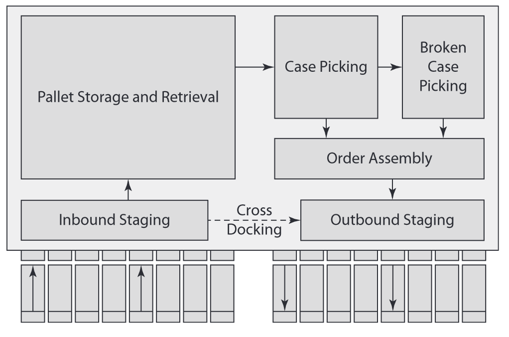
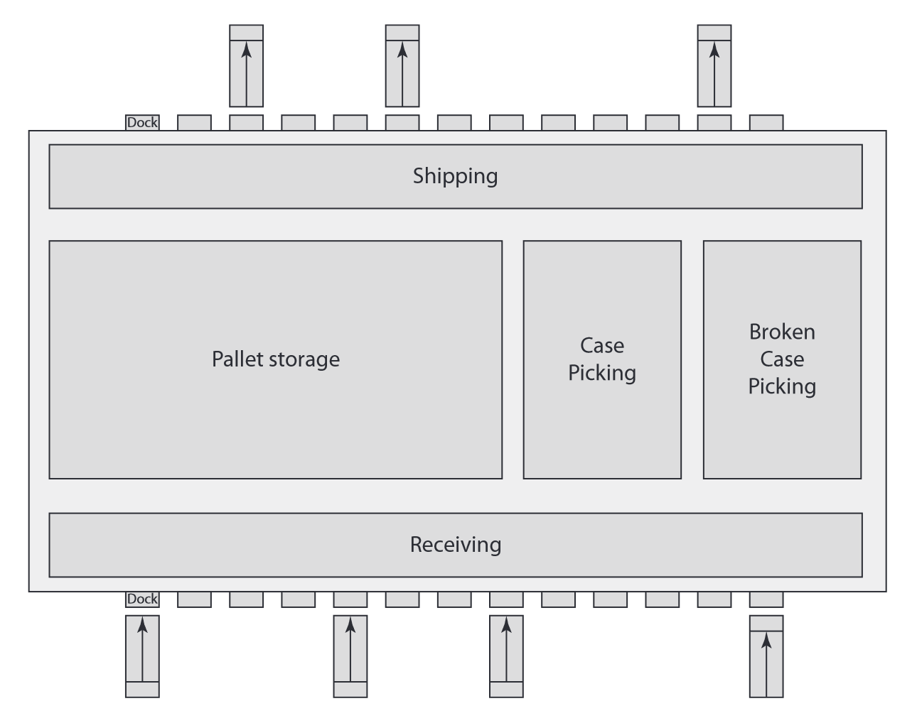
U-shaped, straight-through, modular-spine, and multi-story flow paths work in isolation or in conjunction with one another to form the large majority of warehouse flow paths.

U-shaped, straight-through, modular-spine, and multi-story flow paths work in isolation or in conjunction with one another to form the large majority of warehouse flow paths.

An example U-shaped warehouse flow design is shown in Figure 9.9. Products flow in at receiving and move to receiving staging, pallet storage, case picking, broken-case picking, order assembly, and shipping. A U-shaped flow design yields high utilization of dock resources because receiving and shipping can share dock doors; facilitates cross-docking because receiving and shipping docks are adjacent; yields high lift-truck utilization because put-away and retrieval trips are easily combined and fast-moving items can be stored near both docks; allows expansion in three directions; and provides excellent security because a single side of the building is used for entry and exit. With these inherent advantages, U-shaped flow design is the benchmark against which all other flow designs should be compared.

The straight-through configuration lends itself to warehouse operations attached to factories, with receipts arriving directly from production lines; to pure cross-docking facilities, sometimes referred to as flow-through facilities; or to operations in which peak receiving and shipping times coincide. The major disadvantage is that the design does not lend itself to ABC storage and dual-command trips.

A modular-spine design uses a large material-handling spine to connect independent buildings dedicated to specific warehouse activities in large-scale warehousing and distribution environments. Examples include a rack-supported building for a unit-load automated storage and retrieval system; an air-conditioned building for customizing operations such as monogramming, pricing, and marking; a building dedicated to returns processing; and a shipping building equipped with high-speed sorting equipment.

Multistory distribution buildings are necessary when land is extremely scarce. They are the least desirable of the flow-path alternatives because of the material-handling difficulties and bottlenecks encountered in moving merchandise between floors.

— World-Class Warehousing and Material Handling (Frazelle 2016, 301–4).

U-Shaped flow

High utilization of dock resources (receiving and shipping can share dock doors).
Easier cross-docking (adjacent receiving and shipping docks).
High lift-truck utilization:
- put-away and retrieval trips are easily combined.
- fast-moving items closest to the receiving and shipping docks.
Expansion opportunities in three directions.
Higher security (entry and exit at the single side of the building).

Figure 18: Products flow in at receiving and move to receiving staging, pallet storage, case picking, broken-case picking, order assembly, and shipping (Frazelle 2016)

An example U-shaped warehouse flow design has products flow in at receiving and move to receiving staging, pallet storage, case picking, broken-case picking, order assembly, and shipping. A U-shaped flow design has several advantages:

It yields high utilization of dock resources because receiving and shipping can share dock doors.

It facilitates cross-docking because the receiving and shipping docks are adjacent.

It yields high lift-truck utilization because put-away and retrieval trips are easily combined and the locations closest to the docks naturally house fast-moving items.

It allows expansion in three directions.

It provides excellent security because a single side of the building is used for entry and exit.

With these inherent advantages, U-shaped flow design is the benchmark against which all other flow designs should be compared.

— World-Class Warehousing and Material Handling (Frazelle 2016, 300–301).

Straight-through I-shaped flow design

Favors operations where the warehouse

is attached to factories (receipts arriving from production lines).
is a cross-docking/flow-through facility.
has coinciding peak receiving and shipping times.

Disadvantages:

Hard to implement ABC storage and dual-command¹ trips.

Figure 19: Straight-through flow design (Frazelle 2016)

Modular-spine flow design

Uses a large material-handling spine to connect independent buildings.

Standalone buildings are dedicated to specific warehouse activities in large-scale warehousing and distribution environments. Examples:
- rack-supported buildings for a unit-load automated storage and retrieval system (ASRS);
- air-conditioned building for customizing operations such as monogramming, pricing, and marking;
- building dedicated to returns processing;
- shipping building equipped with high-speed sorting equipment.

Figure 20: Modular-spine flow design (Frazelle 2016)

References

Aussaresse, S. 2023. “Warehousing Trends and Innovations: Best Practices.” BSc thesis, University of Twente, Industrial Engineering; Management. https://purl.utwente.nl/essays/96629.

Baker, Peter, and Marco Canessa. 2009. “Warehouse Design: A Structured Approach.” European Journal of Operational Research 193 (2): 425–36. https://doi.org/10.1016/j.ejor.2007.11.045.

Frazelle, Edward. 2016. World-Class Warehousing and Material Handling. Second Edition. McGraw-Hill Education.

Muther, Richard, and Lee Hales. 2015. Systematic Layout Planning. 4th ed. Management & Industrial Research Publications. https://richardmuther.com/wp-content/uploads/2016/07/Systematic-Layout-Planning-SLP-4th-edition-soft-copy.pdf.

Richard Muther. 2005. Overview of Systematic Layout Planning (SLP). https://richardmuther.com/wp-content/uploads/2014/06/RMA-1146-SLP-Overview-Mfg.pdf.

Richards, Gwynne. 2014. Warehouse Management: A Complete Guide to Improving Efficiency and Minimizing Costs in the Modern Warehouse. Second edition. Kogan Page Limited.

Rouwenhorst, Bart, Bert Reuter, Volker Stockrahm, Geert-Jan van Houtum, Rob Mantel, and Willem H. M. Zijm. 2000. “Warehouse Design and Control: Framework and Literature Review.” European Journal of Operational Research 122 (3): 515–33. https://doi.org/10.1016/S0377-2217(99)00020-X.

The Raymond Corporation. 2018. Storage Space Efficiency Guide: A Demonstration in Space. Brochure. The Raymond Corporation. https://www.raymondcorp.com/forklifts/orderpickers/-/media/0f1598ebec4e43feb77f9a5d1a074898.ashx.

Tompkins, James A., ed. 2010. Facilities Planning. 4th ed. J. Wiley.