Warehouse storage optimization: Inventory management

Inventory is money sitting around in a different form. Rhonda Abrams

🧠 Learning objectives

• Understand the fundamental differences among approaches to managing inventory.
• Describe the rationale and logic behind the economic order quantity (EOQ) approach to inventory decision making.
• Determine a product EOQ under conditions of certainty and uncertainty.

“after reading this chapter, you should be able to do the following: - Appreciate the role and importance of inventory in the economy. - List the major reasons for carrying inventory. - Discuss the major types of inventory, their costs, and their relationships to inventory decisions. - Understand the fundamental differences among approaches to managing inventory. - Describe the rationale and logic behind the economic order quantity (EOQ) approach to inventory decision making, and be able to solve some problems of a simple nature. - Understand alternative approaches to managing inventory—just-in-time (JIT), materials requirement planning (MRP), distribution requirements planning (DRP), and vendor-managed inventory (VMI). - Explain how inventory items can be classified. - Know how inventory will vary as the number of stocking points change. - Make needed adjustments to the basic EOQ approach to respond to several special types of applications.”

— Supply Chain Management: A Logistics Perspective (Coyle et al. 2020, 287).

What is inventory?

• Stock or store of goods:
  • Raw materials, work-in-progress (WIP), finished goods.
  • Maintenance, repair, and operating (MRO) supplies.

“Stock or store of goods” is the slide’s concise phrasing of OpenStax’s definition below. The first three categories identify where inventory sits in a production flow. MRO supplies support the operation itself rather than becoming part of the finished product.

“A firm’s inventory is the supply of goods it holds for use in production or for sale to customers.”

— Introduction to Business (Gitman et al. 2018, sec. 10.4, heading “Inventory Management: Not Just Parts”).

“Your production system will involve planning for inventory. Raw materials inventory is material that you have received from suppliers at the start of your production process, and finished goods inventory is material at the end of the production process that you can sell to customers. Partially assembled products between manufacturing steps are called work-in-process (WIP, pronounced whip) inventory.”

— Supply Chain Management For Dummies (Stanton 2023, 64, sec. “Planning Your Production Systems”).

“Generics are low-risk, low-value items and services that typically do not enter the final product. Items such as office supplies and maintenance, repair, and operating items (MRO) are examples of generics. The administrative and acquisition processing costs are more significant than the purchase price of generics, and, for some generics, the administration and processing costs may exceed the price paid for the item or service. The strategic procurement priority for generics is to streamline the procurement process to reduce the associated costs relating to acquisition. For example, the use of purchasing cards (corporate credit cards) helps to reduce the number of checks written and the administrative costs associated with check payment, bank verification, etc.”

— Supply Chain Management: A Logistics Perspective (Coyle et al. 2020, 143, sec. “Quadrant Technique”).

Why keep inventory?

• To meet customer demand (cycle stock)
• To buffer against uncertainty in demand or supply (safety stock)
• To allow economic purchase orders (lot size inventory)
• To allow flexibility in production scheduling (anticipation inventory)
• To hedge against price increases or shortages (speculative inventory)
• To decouple supply from demand (pipeline inventory)

The six labels on the slide are a course synthesis of several inventory mechanisms; they are not a verbatim taxonomy from Coyle. Read each row through the more specific source concepts below.

Cycle stock and economic lots. Cycle stock arises when procurement, transportation, or production is batched to capture scale economies. It can support demand between replenishments, but the defining mechanism here is the batch decision and its cost trade-off.

“Batching economies or cycle stocks usually arise from three sources—procurement, production, and transportation. Scale economies are often associated with all three, which can result in the accumulation of inventory that will not be used or sold immediately—which means some cycle stock or inventory will be used up or sold over some period of time.

In the procurement area, it is not unusual for a seller to have a schedule of prices that reflects the quantity purchased. In other words, larger purchased volumes result in lower prices per unit and vice versa. Purchase discounts are also prevalent for personal consumption items. For example, buying a package of 12 rolls of paper towels at Sam’s Club would result in a lower price per roll than if the 12 rolls were bought separately. When the larger package is purchased, cycle stock is created. What is not consumed immediately will have to be stored. When organizations buy raw materials and supplies, particularly in our global economy, they are often offered price discounts for larger quantities. The tradeoff logic that was mentioned earlier suggests that the price discount savings have to be compared to the additional cost of carrying inventory.

A related discount situation occurs with transportation services. Transportation firms usually offer rate or price discounts for shipping larger quantities. In the motor carrier industry, a common example is the lower rate or price per pound for shipping truckload quantities versus less-than-truckload quantities. The motor carrier saves money in pick-up, handling, and delivery costs with the truckload shipment, and these are reflected in a lower rate or price to the shipper. The larger shipment quantities to justify the discount have the same effect as the purchase quantities—that is, cycle stocks. The tradeoff requirement is the same. Do the costs savings from the larger shipment offset the additional inventory carrying cost?

The third batching economy is associated with production. Many organizations feel that their production costs per unit are substantially lower when they have long production runs of the same product. Long production runs decrease the number of changeovers to a production line but increase the amount of cycle stock that must be stored until sold.”

— Supply Chain Management: A Logistics Perspective (Coyle et al. 2020, secs. 9–3a, pp. 292–293).

Safety stock. This is the direct buffer against uncertainty in demand, supply lead time, and transportation reliability.

“All organizations are faced with uncertainty. On the demand or customer side, there is usually uncertainty in how much customers will buy and when they will buy it. Forecasting demand is a common approach to resolving demand uncertainty, but it is never completely accurate. On the supply side, there might be uncertainty about obtaining what is needed from suppliers and how long it will take for the fulfillment of the order. Uncertainty can also arise from transportation providers in terms of receiving reliable delivery. The net result of uncertainty is usually the same: organizations accumulate safety stock to buffer themselves against stockouts. The challenge and analysis are different for safety stock than for cycle stock; safety stock is much more complex and challenging to manage because it is redundant inventory.”

— Supply Chain Management: A Logistics Perspective (Coyle et al. 2020, secs. 9–3b, pp. 293–294).

Stanton’s restaurant example makes the demand–lead-time interaction concrete:

“Suppose that you run a fast-food restaurant. You know that it’s very important to never, ever run out of French fries. You have to decide how many French fries to keep in inventory. (The only way to guarantee that you’ll never run out of French fries would be to have an infinite amount of inventory, which would be silly!) In order to decide how much inventory to carry you need to understand both demand (how much your customers are going to buy) and supply. You can start by looking at demand. How much do your customers buy in an average week? How much did they buy in your best week ever? Then you can look at supply. If you know that your suppliers can ship a load of French fries in 24 hours, you don’t need to keep much inventory in your restaurant. But if it takes your supplier a week to send you a new shipment, you probably need to have more inventory on hand as a buffer against a surprise spike in demand.”

— Supply Chain Management For Dummies (Stanton 2023, 115).

Pipeline and work-in-process stock. Goods remain inventory while moving or waiting within production. These stocks decouple stages in time, but their cost grows with elapsed time.

“The time associated with transportation (e.g., supplier to manufacturing plant) and with the manufacture or assembly of a complex product (e.g., automobile) means that even while goods are in motion, an inventory cost is associated with the time period. The longer the time period is, the higher the cost will be.

The time period for in-transit inventory and work-in-process (WIP) inventory should be evaluated in terms of the appropriate tradeoffs. The various transportation modes available for shipping freight have different transit time lengths, transit time variability, and damage rates. The rates or prices charged by carriers in the different modes reflect these differences in service.

Finally, WIP inventories are associated with manufacturing. Significant amounts of inventory can be accumulated in manufacturing facilities, particularly in assembly operations such as automobiles and computers. The length of time WIP inventory sits in a manufacturing facility waiting to be included in a particular product should be carefully evaluated in relationship to scheduling techniques and the actual manufacturing or assembly technology.”

— Supply Chain Management: A Logistics Perspective (Coyle et al. 2020, secs. 9–3c, pp. 294–296).

Seasonal and production-flexibility stock. The slide’s “anticipation inventory” row groups production smoothing and seasonality. Coyle calls the resulting category seasonal stock.

“Seasonality can occur in the supply of raw materials, in the demand for finished product, or in both. Organizations that are faced with seasonality issues are constantly challenged when determining how much inventory to accumulate. Organizations that process agriculture products are a good example of supply seasonality. While the supply of the raw material is available during only one part of the year, demand is stable throughout the year. Therefore, the finished product usually has to be stored until it is sold.”

— Supply Chain Management: A Logistics Perspective (Coyle et al. 2020, secs. 9–3d, p. 296).

Speculative or anticipatory stock. The slide’s speculative-inventory row corresponds to hedging against a foreseen supply disruption, shortage, or price increase.

“A fifth reason to hold inventory arises when an organization anticipates that an unusual event might occur that will negatively impact its source of supply. Examples of these events would include strikes, significant raw materials or finished goods price increase, a major shortage of supply because of political unrest or weather, and so on. In such situations, organizations might accumulate inventory to hedge against the risk associated with the unusual event. Again, an analysis should be undertaken to assess the risk, probability, and cost of inventory.”

— Supply Chain Management: A Logistics Perspective (Coyle et al. 2020, secs. 9–3e, p. 296).

Across all six rows, inventory is justified only when its benefit offsets its carrying and risk costs:

“Most organizations will accumulate some level of inventory for very good reasons. In many instances, the inventory cost might be more than offset by savings in other areas. The basic principle is that decisions to accumulate inventory need to be evaluated using a tradeoff framework.”

— Supply Chain Management: A Logistics Perspective (Coyle et al. 2020, secs. 9–3f, p. 297).

Warehouse management vs. inventory management

• Warehouse management
  • Focus: Efficient warehouse operations (storage and movement of goods).
  • Key decisions (related to inventory): Where to store and how to handle items.
  • Goal: Maximize warehouse efficiency and ensure timely order fulfillment.
• Inventory management
  • Focus: Balancing inventory levels to meet customer demand while minimizing costs.
  • Key decisions: When and how much inventory to order.
  • Goal: Maintain optimal inventory levels to avoid stockouts and overstocking.

Tip

Warehouse management can inform inventory management decisions by identifying fast-, medium-, slow-, non-moving, and obsolete stock (Richards 2014; “Warehouse Vs. Inventory” 2025).

“stock management Inventory or stock management and warehouse management tend to be two very distinct roles. Warehouse managers are in a position to advise their inventory colleagues on levels of safety stock and the specific movements and characteristics of particular stock items. However, they tend to stop short of determining stock levels. This function is a major part of a company’s operation and the theories and practices are covered in many books on the subject of inventory management. Although the majority of warehouse managers are not involved directly in the choice, purchase and replenishment of stock, they can play a role in the identification of fast-, medium-, slow-, non-moving and obsolete stock. This can be done using one of the mainstays of a warehouse manager’s armoury – an ABC classification. The information can normally be obtained from the WMS and as mentioned in Chapter 4 a simple spreadsheet can categorize stock items by volume and frequency of sales. A warehouse manager can extend the normal classification to include nonmoving and obsolete stock together with identifying stock that may not require storage in the warehouse but can be despatched direct from the supplier to the end customer where the lead-time is in line with the customer’s requirement.”

— Warehouse Management: A Complete Guide to Improving Efficiency and Minimizing Costs in the Modern Warehouse (Richards 2014, 171).

“The percentages will vary significantly by company and by market sector. Maintenance stores are likely to have a high proportion of their stock in the C to X categories. The goal is to identify the items in the C to X categories and act accordingly. Obsolete or non-moving stock needs to be analysed and one of the following tasks undertaken: ● Return to seller if the contract allows. ● Sell to staff at a discount. ● Sell the item at a highly discounted rate either through normal channels or via companies who specialize in selling overstocks and obsolete items. ● Assess whether it is cost effective to break the item down into its constituent parts. ● Donate to charities. ● Dispose of the product as cheaply as possible. This may incur charges but it will release space to store other faster-moving product in its place. Warehouse Processes from Replenishment to despatch and beyond 173 A quick and easy way of ascertaining whether there is an excess of slowmoving stock in the warehouse is to calculate the stock turn: Stock turn = cost of goods sold ÷ average cost of goods stored or: Annual throughput in units ÷ average number of units held in stock For example, an annual throughput of 1,200,000 units with an average stockholding of 100,000 units gives a stock turn of 12. That is, the stock turns over once per month. A low turn in most operations suggests that stock sits in a warehouse for far too long, implying that the safety stock level has been set too high. Typical examples of stock turn within companies are as follows: 150 +: world class using just-in-time techniques; 120 +: chilled foods; 18 +: retail; 10–30: European manufacturing; <3: maintenance stores. The higher the figure, the better the company is performing in terms of inventory management. Maintenance stores will always have low stock turns through having to hold stock in case of breakdown.”

— Warehouse Management: A Complete Guide to Improving Efficiency and Minimizing Costs in the Modern Warehouse (Richards 2014, 172).

“Definition and Key Concepts Warehouse management is the process of efficiently managing and controlling all aspects of a warehouse’s operations. It encompasses inventory tracking, order fulfillment, and storage optimization to ensure that products are stored in the right place, picked and packed accurately, and delivered to customers on time. Key components of warehouse management include: Inventory Tracking: Monitoring the movement and storage of goods within the warehouse. Order Fulfillment: Ensuring that customer orders are processed and shipped accurately and promptly. Storage Optimization: Utilizing warehouse space efficiently to maximize storage capacity and accessibility. Warehouse Management System (WMS): A software solution designed to streamline and optimize warehouse operations. A WMS helps manage inventory, track shipments, and improve overall warehouse efficiency. Warehouse management focuses on ensuring that warehouse operations are efficient, cost-effective, and compliant with regulatory standards. By implementing a robust warehouse management system, businesses can enhance their warehouse processes, reduce handling times, and improve logistics.”

— Warehouse vs. Inventory: Their Roles and Differences (“Warehouse Vs. Inventory” 2025, sec. “Definition and Key Concepts”).

“Benefits of Effective Inventory Management Effective inventory management offers numerous benefits that can significantly impact a business’s bottom line and operational efficiency. These benefits include: Greater Inventory and Order Accuracy: Reduces discrepancies between recorded and actual stock levels, ensuring that inventory data is reliable. Boosted Efficiency: Streamlines inventory processes, reducing the time and effort required to manage stock. Lower Overhead Costs: Minimizes storage costs and reduces the need for excess inventory, freeing up capital for other uses. Faster Inventory Turns: Increases the rate at which inventory is sold and replaced, improving cash flow and reducing holding costs. Increased Customer Satisfaction: Ensures that products are available when customers need them, leading to higher satisfaction and loyalty. Better Decision-Making: Provides valuable data and insights that help businesses make informed decisions about purchasing, production, and sales. By implementing effective inventory management strategies, businesses can optimize their inventory levels, reduce waste, and improve their overall supply chain operations. This not only enhances inventory accuracy but also streamlines supply chain processes, ultimately leading to improved customer satisfaction and operational excellence.”

— Warehouse vs. Inventory: Their Roles and Differences (“Warehouse Vs. Inventory” 2025, sec. “Benefits of Effective Inventory Management”).

“Understanding Warehouse Management The Role Of A Warehouse A warehouse is a storage facility that efficiently stores and protects goods until they are needed for distribution or sale. It plays a crucial role in the supply chain by managing inventory, fulfilling orders, and facilitating distribution. Inventory management and warehouse operations are closely related, working together to ensure efficient movement, storage, and control of stock. The Role Of Inventory Inventory, encompassing all goods and materials held by a business for sale or production, plays a pivotal role in maintaining the seamless operation of supply chains across retail, trade, and manufacturing sectors. Understanding the distinctions between inventory management and warehouse management is crucial for effective inventory and warehouse operations.”

— Warehouse vs. Inventory: Their Roles and Differences (“Warehouse Vs. Inventory” 2025, sec. “Understanding Warehouse Management”).

Inventory management

How to keep the right amount of inventory on hand?

• Too much inventory: wasting capital (excess inventory and holding costs).
• Too little inventory: stockouts (lost sales, unhappy customers).

“Trying to keep the right amount of inventory on hand is a tricky business. Keep too much inventory, and you’re wasting money by tying up working capital. Keep too little inventory, and you’ll miss out on revenue because you won’t have anything to sell to your customers. Two of the most important decisions you can make are when to order more inventory and how much to order. The approach you use to make that decision is called your inventory policy. Start with the question of when to order more inventory from your suppliers. You may need to place an order when your current inventory levels drop below a certain level, in which case the current inventory level is the trigger for your inventory policy. Or you may want to order inventory on a set schedule, such as once a week, in which case your inventory policy is built on periodic orders. Triggering orders based on inventory levels is usually more efficient than periodic orders. But suppliers often schedule deliveries periodically because it is more convenient for them. So you need to understand the dynamics of a particular supply chain to make the best decision about which inventory trigger to use.”

— Supply Chain Management For Dummies (Stanton 2023, 122).

Key differences between inventory management approaches

• Dependent Demand vs. Independent Demand
• Pull versus Push
• System-wide versus Single-facility

Major inventory management approaches:

• Just-in-time (JIT)
• Materials Requirements Planning (MRP)
• Distribution Requirements Planning (DRP)
• Vendor-managed Inventory (VMI)
• Economic Order Quantity (EOQ)

Given the various approaches to managing inventory that are available and used today, it is important to know how they differ. These differences include dependent versus independent demand, pull versus push, and system-wide versus single-facility solutions to inventory management decisions.

Demand for a given inventory item is termed independent when such demand is unrelated to the demand for other items. Conversely, demand is defined as dependent when it is directly related to, or derives from, the demand for another inventory item or product. For example, the demand for a laptop computer is independent, while the demand for its computer chip is dependent. This dependency can be vertical (the laptop needs the chip for assembly) or horizontal (the laptop needs an instruction manual for final delivery to the customer).

For many manufacturing processes, basic demand for raw materials, component parts, and subassemblies depends on the demand for the finished product. In contrast, the demand for end-use items, which are typically sold to a customer, is independent of the demand for any other higher-order manufactured item. Developing inventory policies for items exhibiting independent demand requires forecasts for those items. Forecasting is less relevant for items having dependent demand because the required quantities depend entirely on demand for the end-use product. Once demand for end-use items is forecast, determining demand for dependent items requires calculations based on the bill of materials. JIT, MRP, and manufacturing resource planning are usually associated with dependent-demand items. DRP generally involves independent-demand items. EOQ and vendor-managed inventory apply to both independent- and dependent-demand items.

The pull approach relies on customer orders to move product through a logistics system, while the push approach uses inventory-replenishment techniques in anticipation of demand. Pull systems can respond quickly to abrupt changes in demand because they produce to an order and hold little, if any, finished-goods inventory. Push systems produce to inventory in anticipation of demand, which limits their ability to adapt to changing volumes and preferences. Pull systems usually use short-term forecasts, allowing flexibility. Push systems use longer-term forecasts that permit manufacturing scale economies but result in high finished-goods inventories. These inventories can make shelf life a problem in push systems, whereas it is not an issue for pull systems.

JIT is characteristically a pull system because organizations order more inventory only when the amount on hand reaches a minimum level. MRP and MRP II are typically push based because they generate required-material lists from a master production schedule. DRP is also push based because it allocates available inventory to meet market demand. VMI uses preset reorder points, economic order quantities, and inventory levels in customers’ warehouses to generate replenishment orders; because the customer does not place the order, VMI can be considered a push approach. EOQ is generally a pull approach, but contemporary applications may include push elements. Many EOQ-based systems are hybrids containing both pull- and push-based strategies.

A final issue is whether the selected approach represents a system-wide solution or is specific to a single facility. A system-wide approach plans and executes inventory decisions across multiple nodes. MRP and DRP are typically system-wide approaches because they plan inventory releases and receipts between multiple shipping and receiving points. A single-facility approach plans and executes shipments and receipts between one shipping point and one receiving point. EOQ and JIT are normally single-facility solutions. MRP and DRP are usually employed to plan system inventory movements, while EOQ and JIT execute these plans at the facility level. VMI can plan system-wide replenishment and execute replenishment at a single facility.

— Supply Chain Management: A Logistics Perspective (Coyle et al. 2020, 312–14).

Dependent vs. independent demand

Independent

• Unrelated to the demand for other items.
• Demand for end-use items sold to a customer does not depend on a higher-order manufactured item.
• Inventory policy depends on demand forecasting.

Dependent

• Demand directly related to, or derives from, the demand for another inventory item or product
  • Raw materials, component parts, sub-assemblies depend on the demand for the finished product (e.g., computer chip).
• Inventory policy depends on demand forecasting for the higher-order manufactured item.

“Dependent Versus Independent Demand

Demand for a given inventory item is termed independent when such demand is unrelated to the demand for other items. Conversely, demand is defined as dependent when it is directly related to, or derives from, the demand for another inventory item or product. For example, the demand for a laptop computer is independent, while the demand for its computer chip is dependent. This dependency can be vertical (the laptop needs the chip for assembly) or horizontal (the laptop needs an instruction manual for final delivery to customer). So, for many manufacturing processes, basic demand for raw materials, component parts, and subassemblies depends on the demand for the finished product. In contrast, the demand for the end-use items, which are typically sold to a customer, is independent of the demand for any other higher-order manufactured item. An important point to remember is that developing inventory policies for items exhibiting independent demand requires that forecasts be developed for these items. Alternatively, forecasting is less relevant for items having dependent demand since the required quantities for these items depend entirely on the demand for the end-use product. So, once the difficult task of forecasting demand for end-use items is completed, determining the demand for dependent items requires simple calculations based on the bill of materials for that item. Of the approaches to inventory management that will be discussed, JIT, MRP, and manufacturing resource planning (MRP II) are usually associated with items having dependent demand. Alternatively, DRP generally involves the movement of items having independent demand. The EOQ and vendor-managed inventory approaches apply to both independent and dependent demand items.”

— Supply Chain Management: A Logistics Perspective (Coyle et al. 2020, 313).

Dependent vs. independent demand

Pull vs. push

Pull approach

• Relies on customer orders to move product through the logistics system
• Can respond quickly to sudden demand changes
  • Little or no finished goods inventory
  • Postponement of value addition
• Run on short-term forecasts (flexibility to adapt to demand swings)
• Examples: JIT, EOQ

Push approach

• Inventory replenishment techniques in anticipation of demand (proactive)
  • Limited ability to adapt to changing demand volumes and preferences
• Longer-term forecasts
  • Scale economies in manufacturing
  • High finished goods inventories (impacted by shelf life)
• Examples: VMI

EOQ-based systems in evidence today are hybrid approaches that include elements of both pull- and push-based strategies.

“Pull Versus Push

The “pull” approach relies on customer orders to move product through a logistics system, while the “push” approach uses inventory replenishment techniques in anticipation of demand to move products. For example, Dell has traditionally used the pull approach for the assembly of its computers. With little or no finished goods inventory for computers, Dell waits for a customer order for a computer before it begins assembly. Recently, however, Dell began selling a limited line of its computers through Walmart retail stores. To do this, Dell employs the push model to anticipate future demand, assemble computers to inventory, and move them through its logistics system into Walmart stores. A principal attribute of pull systems is that they can respond quickly to sudden or abrupt changes in demand because they produce to an order and have very little, if any, finished goods inventory. This is especially true for products where the final addition of value can be postponed. Alternatively, push systems produce to inventory in anticipation of demand, thus making their ability to adapt to changing demand volumes and preferences limited. Pull systems usually run on short-term forecasts, allowing them the flexibility to adapt to swings in demand. On the other hand, push systems use longer-term forecasts that allow for scale economies in manufacturing but result in high finished goods inventories. These high levels of finished goods inventories can make shelf life a problem in push systems, while this is not an issue for pull systems. Characteristically, JIT is a pull system since organizations place orders for more inventory only when the amount on hand reaches a certain minimum level, thus “pulling” inventory through the logistics system as needed. Having established a master production schedule, MRP develops a time-phased approach to inventory scheduling receipt. Because they generate a list of required materials in order to assemble or manufacture a specific amount of finished products, MRP and MRP II approaches are typically push based, although some examples can be offered that they are also pull based. Similar to these, but on the outbound or physical distribution side of logistics, DRP involves the allocation of available inventory to meet market demands. Thus, DRP is also a push-based strategy. VMI uses preset reorder points and economic order quantities along with on-hand inventory levels in customers’ warehouses to generate replenishment orders. Because the customer is not placing a replenishment order, VMI can be considered a push approach.

Finally, the EOQ approach is generally a pull approach, but applications today include elements of the push approach as well. While this permits the EOQ technique to be reactive when necessary, it also allows the preplanning of certain inventory decisions in a proactive, or push, manner. In fact, many EOQ-based systems in evidence today are hybrid approaches that include elements of both pull- and push-based strategies.”

— Supply Chain Management: A Logistics Perspective (Coyle et al. 2020, 313).

Pull vs. push

What is the difference between push and pull approaches?

In inventory management, the push and pull approaches refer to different strategies for managing the flow of goods through the supply chain.

Push Approach: In the push approach, inventory decisions are based on forecasts and production schedules. Goods are produced or purchased in advance and pushed through the supply chain to downstream locations such as warehouses and retailers. The focus is on anticipating demand and pushing products to meet that anticipated demand.

Pros:

• Helps meet anticipated demand and ensures product availability.
• Suitable for products with stable demand patterns or long production lead times.
• Can take advantage of economies of scale in production.

Cons:

• Prone to overstocking or understocking if demand forecasts are inaccurate.
• Can result in higher inventory carrying costs and potential obsolescence.
• Lack of flexibility to respond to sudden changes in customer demand.

Pull Approach: In the pull approach, inventory decisions are based on actual customer demand. Products are not produced or procured until there is a confirmed order or a signal from the downstream customer. The focus is on reacting to demand signals and pulling products through the supply chain as needed. Pros:

• Reduces the risk of overstocking and minimizes inventory carrying costs.
• Enables a more flexible response to changes in customer demand.
• Helps to align production with actual demand, reducing waste and obsolescence.

Cons:

• Requires efficient communication and coordination across the supply chain to ensure timely responses to customer demand.
• May lead to stockouts if demand spikes or supply chain disruptions occur.
• Can be challenging for products with long lead times or complex manufacturing processes.

Overall, the choice between the push and pull approaches depends on factors such as the nature of the product, demand patterns, lead times, and the level of coordination and visibility within the supply chain. Many organizations use a combination of both approaches, often referred to as a hybrid or lean inventory management strategy, to strike a balance between meeting customer demand and minimizing inventory-related costs.

System-wide vs. single-facility solutions

• System-wide approach. Plan inventory releases and receipts between multiple shipping and receiving points in the logistics system. Example:
  • MRP (Materials Requirements Planning)
  • DRP (Distribution Requirements Planning)
  • VMI (Vendor-Managed Inventory)

Single-facility approach. Release orders from a single facility (e.g., DC) to a specific supplier for inventory replenishment. Example:

• EOQ (Economic Order Quantity)
• JIT (Just-In-Time)
• VMI (Vendor-Managed Inventory)

“System-Wide Versus Single-Facility Solutions A final inventory management issue is whether the selected approach represents a system-wide solution or whether it is specific to a single facility, such as a distribution center. Basically, a system-wide approach plans and executes inventory decisions across multiple nodes in the logistics system. MRP and DRP are typically system-wide approaches to managing inventory. Both approaches plan inventory releases and receipts between multiple shipping and receiving points in the network. On the other hand, a single-facility approach plans and executes shipments and receipts between a single shipping point and receiving point. EOQ and JIT are normally considered single-facility solutions. Both release orders from a single facility to a specific supplier for inventory replenishment. Usually, MRP and DRP are employed to plan system inventory movements, and EOQ and JIT are used to execute these plans at a single-facility level. VMI can be used to plan system-wide replenishment as well as execute replenishment on a single-facility basis.”

— Supply Chain Management: A Logistics Perspective (Coyle et al. 2020, 314).

System-wide vs. single-facility solutions

Inventory policy decisions

Decisions to set an inventory policy:

• How much to order?
  • Order enough to cover demand for a certain period (e.g., one week, one month).
  • Order a fixed amount each time (e.g., EOQ).
• When to order?
  • Order periodically, on a set schedule (often more convenient for suppliers).
  • Order when inventory levels drop below a certain level (triggering orders).

An inventory policy separates the quantity decision from the timing decision. A fixed-order-quantity policy keeps the replenishment amount constant and lets a stock-level trigger determine the time of the order. A fixed-order-interval policy keeps the review schedule constant and lets the replenishment amount depend on the stock found at review.

“As its name implies, the fixed order quantity model involves ordering a fixed amount of product each time reordering takes place. The exact amount of product to be ordered depends on the product’s cost and demand characteristics and on relevant inventory carrying and reordering costs.”

— Supply Chain Management: A Logistics Perspective (Coyle et al. 2020, 314, sec. 9-5c).

“The second form of the basic approach is the fixed order interval approach to inventory management, also called the fixed period or fixed review period approach. In essence, this technique involves ordering inventory at fixed or regular intervals; generally, the amount ordered depends on how much is in stock and available at the time of review. Organizations usually count inventory near the interval’s end and base orders on the amount on hand at that time.”

— Supply Chain Management: A Logistics Perspective (Coyle et al. 2020, 330–31, sec. 9-5e).

Fixed order quantity approach (condition of certainty)

• Involves ordering a fixed amount of product each time reordering takes place.
• Exact amount of product to be ordered depends on
  • the product’s cost and demand characteristics
  • relevant inventory carrying and reordering costs

The model fixes the replenishment quantity, but the value of that quantity still depends on item economics and demand. This is why the later EOQ formulation needs demand, unit value, carrying cost, and ordering cost as separate inputs.

“As its name implies, the fixed order quantity model involves ordering a fixed amount of product each time reordering takes place. The exact amount of product to be ordered depends on the product’s cost and demand characteristics and on relevant inventory carrying and reordering costs.”

— Supply Chain Management: A Logistics Perspective (Coyle et al. 2020, 314, sec. 9-5c).

What is Economic Order Quantity (EOQ)?

• Mathematical approach to calculating lot size proposed first by Harris (1913; see historical context in Erlenkotter 1990).
• Balances the cost of placing an order against the cost of holding inventory.
• Formula requires tweaking in the real-world:
  • Packaging (e.g., you need X items, but pallet is sold with X+Y)
  • Seasonal demand
  • Promotions
  • Quantity discounts
  • Variable lead times

EOQ is historically a square-root lot-size model. Its central idea is to balance inventory carrying cost against ordering cost. The slide’s packaging, seasonal-demand, promotion, discount, and variable-lead-time examples are practical reasons why a simple model’s certainty assumptions may need modification.

“Ford Whitman Harris first presented the familiar economic order quantity (EOQ) model in a paper published in 1913. Even though Harris’s original paper was disseminated widely, it apparently was unnoticed for many years before its rediscovery in 1988. During this period much confusion developed over the origin of the EOQ model.”

“Today the EOQ model is so well known that we accept its basic structure as obvious. In 1913, however, it was a modeling achievement of classical elegance. The simple square-root formula for the optimal order quantity followed directly from Harris’s assumption of a continuous constant rate for demand and his recognition of the need to balance intangible inventory costs against the tangible costs for ordering.”

— Ford Whitman Harris and the Economic Order Quantity Model (Erlenkotter 1990, 937–38).

“Every manufacturer is confronted with the problem of finding the most economical quantity to manufacture in putting through an order. This is a general problem and admits of a general solution, and, however much it may be advisable to exercise judgment in a particular case, such exercise of judgment will be assisted by a knowledge of the general solution.”

“The writer has seen the practical workings of a first-class stock system and does not wish to be understood as claiming that any mere mathematical formula should be depended upon entirely for determining the amount of stock that should be carried or put through on an order. This is a matter that calls, in each case, for a trained judgment, for which there is no substitute. There are many other factors of even more importance than those given in this discussion. But in deciding on the best size of order, the man responsible should consider all the factors that are mentioned. While it is perfectly possible to estimate closely enough what effect these factors will have, the chances are many mistakes costing money will be made. Hence, using the formula as a check, is at least warranted. Given the theoretically correct result, it is easy to apply such correction factors as may be deemed necessary.”

— How Many Parts to Make at Once (Harris 1913, 947).

“Given the assumptions listed, the simple EOQ model considers only two basic types of cost: inventory carrying cost and ordering cost. The simple model arrives at an optimum decision that analyzes the tradeoffs between these two costs. If the model focused only on inventory carrying cost, which varies directly with changes in order quantity, the order quantity would be as small as possible. If the model considered only ordering cost, large orders would decrease total order costs, and small orders would increase total order costs. The lot size decision attempts to minimize total cost by reaching a compromise between these two costs.”

— Supply Chain Management: A Logistics Perspective (Coyle et al. 2020, 317, sec. “Simple EOQ Model”).

“Much has been written about the number of new products that come on the market each year. Their size, shape, weight, packaging, and other physical dimensions affect the ability of logistics and supply chain systems to move and store the new products. The logistics manager can offer input when marketing is deciding on the physical dimensions of new products to minimize problems. In addition to new products, organizations frequently change established products to improve or maintain sales. Very often, such changes might take the form of new package design and, perhaps, different package sizes. The physical dimensions of products affect the utilization and costs of warehousing and transportation systems such as equipment needed, damage rates, storage ability, use of materials-handling equipment such as conveyors and pallets, industrial packaging, etc.”

“Frustration can mount for logistics managers when faced with a change in a product’s dimensions that makes use of standard-size pallets uneconomical, uses trailer or container space inefficiently, or creates the risk of product damage. These issues may seem somewhat trivial to sales and marketing executives, but they greatly affect an organization’s overall success and profitability in the long run. Collaboration is needed to give logistics managers opportunities for input in these decisions.”

— Supply Chain Management: A Logistics Perspective (Coyle et al. 2020, 68–69, sec. “Product”).

“In the procurement area, it is not unusual for a seller to have a schedule of prices that reflects the quantity purchased. In other words, larger purchased volumes result in lower prices per unit and vice versa. Purchase discounts are also prevalent for personal consumption items. For example, buying a package of 12 rolls of paper towels at Sam’s Club would result in a lower price per roll than if the 12 rolls were bought separately. When the larger package is purchased, cycle stock is created. What is not consumed immediately will have to be stored. When organizations buy raw materials and supplies, particularly in our global economy, they are often offered price discounts for larger quantities. The tradeoff logic that was mentioned earlier suggests that the price discount savings have to be compared to the additional cost of carrying inventory. This is a relatively straightforward analysis, which is discussed later in this chapter. In spite of the framework available for analyzing discount tradeoffs, sometimes organizations just focus on the price savings and do not justify the discount against the additional inventory carrying cost.”

— Supply Chain Management: A Logistics Perspective (Coyle et al. 2020, 293, sec. “Cycle Stock”).

“Within industries faced with seasonal demand patterns, manufacturing is optimized by producing product even though demand for the product does not exist at the time of production. Adding the complexity of production scheduling to accommodate product line growth and brand extensions to this seasonality can result in significantly high inventories to create low manufacturing costs.”

— Supply Chain Management: A Logistics Perspective (Coyle et al. 2020, 297, sec. “Manufacturing”).

“Companies may spend millions of dollars on national advertising campaigns and other promotional practices to improve sales. An organization making a promotional effort to stimulate sales should collaborate with the logistics manager so that appropriate levels of inventory will be available for distribution to the customer. Problems can still occur, even with collaboration, because of the difficulty of forecasting the demand for a new product, but frequent exchange of information can mitigate problems.”

— Supply Chain Management: A Logistics Perspective (Coyle et al. 2020, 69, sec. “Promotion”).

“Most organizations would not operate under conditions of certainty for a variety of reasons. First, consumers usually purchase products somewhat sporadically. The demand rates for many products vary depending on weather, social needs, physical needs, and a whole host of other factors. As a result, the demand for most products varies by day, week, and season.”

“In addition, several factors can affect lead time. For example, transit times can and do change, particularly over long distances, despite transportation provider efforts. Factors such as weather, highway congestion, port congestion, and border stops can make transit times very unreliable. In fact, transit time reliability is a major factor used by organizations when they are making both mode and carrier decisions. Other factors that can cause variations in lead time are order transmittal and processing. Although a significant number of orders today are transmitted electronically, many are still sent through the U.S. Post Office. Mailed orders can be subject to the same unreliability in transit time as mentioned previously. During order processing, factors such as credit blocks and inventory unavailability can cause delays in orders proceeding through the system.”

— Supply Chain Management: A Logistics Perspective (Coyle et al. 2020, 323–24, sec. “Fixed Order Quantity Approach (Condition of Uncertainty)”).

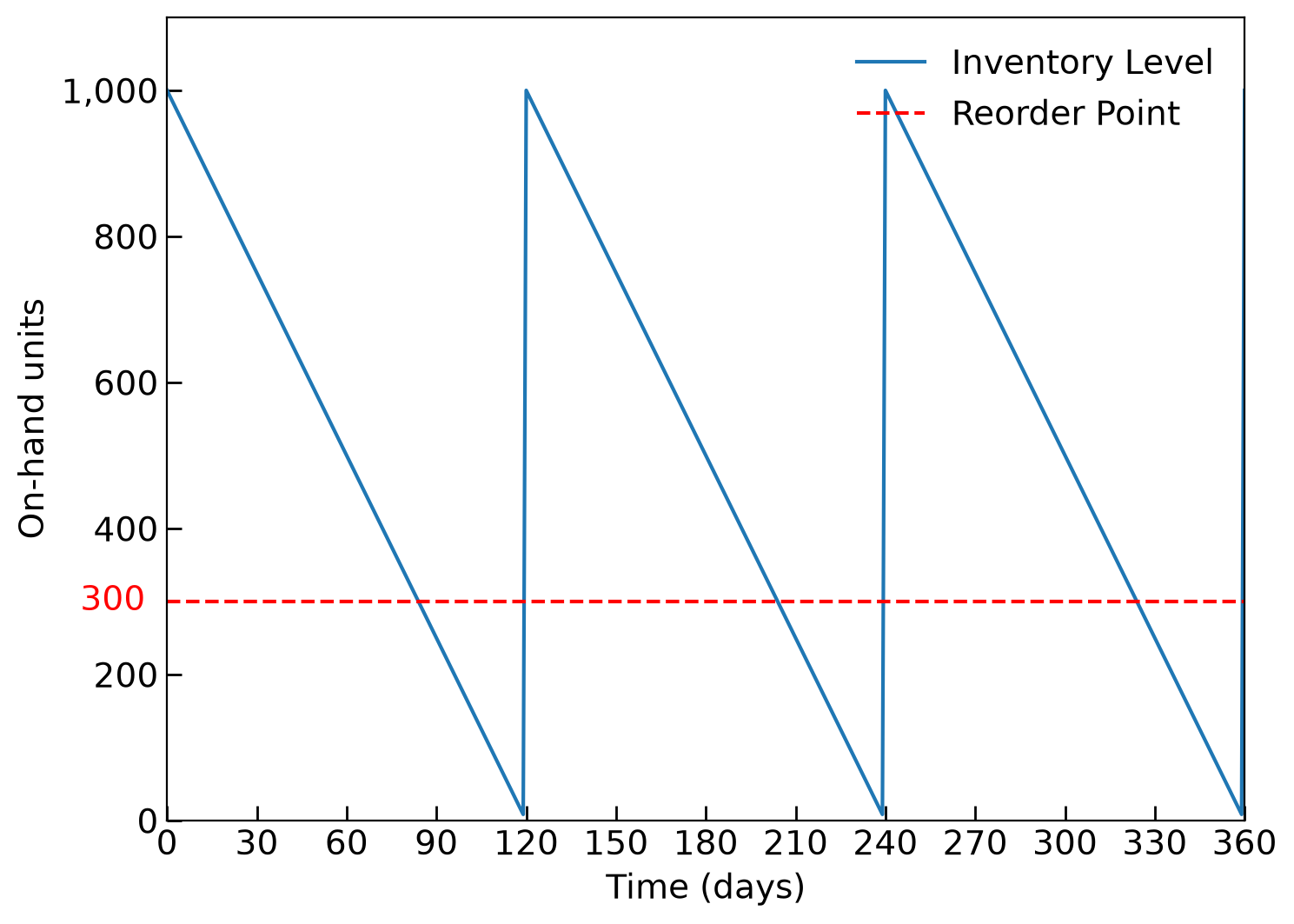
Reorder point

• Minimum stock level to determine when to reorder the fixed order quantity (the EOQ).
• Triggers the next order.
• Quantity depends on:
  • Time to get the new order
  • Demand for the item within lead time
• Example:
  • Lead time new order = 10 days;
  • Demand = 10 units/day;
  • Reorder point = 100 units (10 \(\times\) 10).

The reorder point answers when to replenish. Under certainty, it must cover all demand that occurs during the replenishment lead time; reaching that level triggers the fixed order.

“Organizations using this approach generally needs to develop a minimum stock level to determine when to reorder the fixed quantity. This is called the reorder point. When the number of units of an item in inventory reaches the reorder point, the fixed order quantity (the EOQ) is ordered. The reorder point, then, triggers the next order.”

“The fixed order quantity model is often referred to as the two-bin model. When the first bin is empty, the organization places an order. The amount of inventory in the second bin represents the quantity needed until the new order arrives. Both notions (trigger and bin) imply that an organization will reorder inventory when the amount on hand reaches the reorder point. The reorder point quantity depends on the time it takes to get the new order and on the demand for the item during this lead time. For example, if a new order takes 10 days to arrive and the organization sells or uses 10 units per day, the reorder point will be 100 units (10 days × 10 units/day).”

— Supply Chain Management: A Logistics Perspective (Coyle et al. 2020, 314–15, sec. 9-5c).

Inventory cycles

Figure 1: Fixed order quantity model. Three 120-day inventory cycles beginning with 1,000 units and reorder point of 500 units.

The three curves encode the EOQ tradeoff. Larger order quantities raise average inventory and carrying cost, but reduce the number of annual orders and ordering cost. Their sum reaches its minimum where neither cost can be reduced without increasing the other more.

“Given the assumptions listed, the simple EOQ model considers only two basic types of cost: inventory carrying cost and ordering cost. The simple model arrives at an optimum decision that analyzes the tradeoffs between these two costs. If the model focused only on inventory carrying cost, which varies directly with changes in order quantity, the order quantity would be as small as possible (see Figure 9.6). If the model considered only ordering cost, large orders would decrease total order costs, and small orders would increase total order costs (see Figure 9.7). The lot size decision attempts to minimize total cost by reaching a compromise between these two costs (see Figure 9.8).”

— Supply Chain Management: A Logistics Perspective (Coyle et al. 2020, 317–19, figs. 9.6–9.10).

Simple EOQ Model Assumptions (Pt. 1)

1. A continuous, constant, and known rate of demand
2. A constant and known replenishment or lead time
   • No concerns about stockouts or safety stocks
3. All demand is satisfied
4. A constant price or cost that is independent of the order quantity (i.e., no quantity discounts)
5. No inventory in transit
   • Organization purchases goods on a delivered price basis (purchase price includes transportation costs).

The first five assumptions create a certainty model. Demand and lead time are known, all demand is satisfied, price does not vary with order quantity, and ownership does not create in-transit inventory. These restrictions make the basic EOQ tractable and explain why safety stock and stockouts are absent from this version.

“The following are the basic assumptions of the simple EOQ model:

1. A continuous, constant, and known rate of demand
2. A constant and known replenishment or lead time
3. All demand is satisfied
4. A constant price or cost that is independent of the order quantity (i.e., no quantity discounts)
5. No inventory in transit”

“The first three assumptions are closely related and basically mean that conditions of certainty exist. Demand in each relevant time period (daily, weekly, monthly) is known, and the usage rate is linear over time. The organization uses or depletes inventory on hand at a constant rate and knows the time needed to replenish stock. In other words, the lead time between order placement and order receipt is constant with no variability. As a result, the organization has no need to be concerned about stockouts and safety stock.”

“The fourth assumption (constant costs) essentially means that quantity discounts do not exist. That is, the price of each unit remains the same, regardless of how much is ordered.”

“Assuming that there is no inventory in transit means that the organization purchases goods on a delivered price basis (purchase price includes transportation costs) and sells the goods FOB origin (the buyer pays the transportation costs). On the inbound side, this means that title to the goods does not pass until the buyer receives them. On the outbound side, title passes when the product leaves the shipping point. Under these assumptions, the organization has no responsibility for inventory in transit.”

— Supply Chain Management: A Logistics Perspective (Coyle et al. 2020, 316–17, sec. “Simple EOQ Model”).

Simple EOQ Model Assumptions (Pt. 2)

6. One item of inventory or no interaction between items; multiple items compound mathematical complexity.
7. Infinite planning horizon: constraints are not imposed on the length of the time periods included in the basic model.
8. Unlimited capital: no financial reasons limit the quantity ordered.

The remaining assumptions bound the model’s scope. A basic EOQ calculation treats one independent-demand item at a time, does not stop at a finite planning date, and does not impose a financing limit on the order quantity.

“The sixth assumption means that the simple model is used to order one item of inventory at each order placement. The basic model easily handles the demand for a single, independent demand item with a single price. Introducing the calculation of an economic order quantity for more than one item into the simple model compounds the difficulty of the mathematics.”

“Assumptions seven and eight are most often decisions made outside the logistics area. An infinite planning horizon assumes that constraints are not imposed on the length of the time periods that are included in the basic model. Unlimited capital means that there are no financial reasons to limit the quantity ordered.”

— Supply Chain Management: A Logistics Perspective (Coyle et al. 2020, 316–17, sec. “Simple EOQ Model”).

EOQ Formulation

Table 1: EOQ variables

Symbol	Description
\(R\)	Annual rate of demand (units)
\(Q\)	Quantity ordered (units)
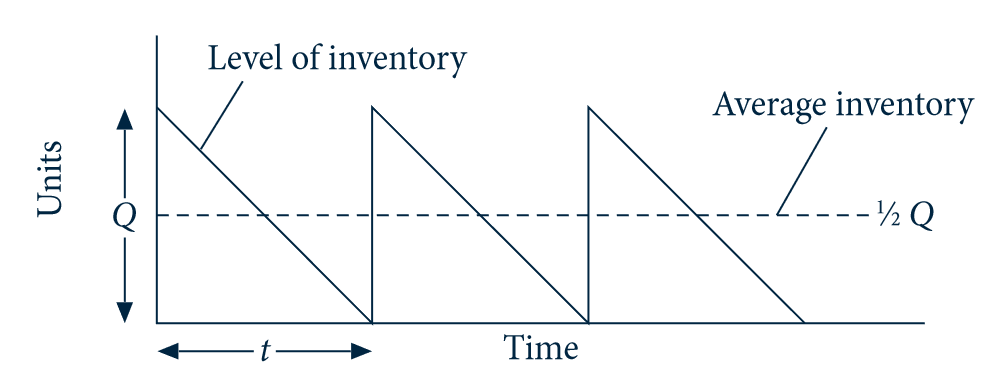
\(\frac{1}{2}Q\)	Avg. number of units during order cycle
\(A\)	Cost of placing an order
\(V\)	Cost of one unit of inventory
\(W\)	Carrying cost/unit of inventory/year (%)
\(S\)	= \(VW\). Inventory carrying cost per unit per year
\(t\)	Order cycle time (days)
\(TAC\)	Total annual cost

Total annual cost adds two opposing terms. Cycle-stock carrying cost is average inventory, \(Q/2\), times unit value \(V\) and annual carrying-rate \(W\). Ordering cost is cost per order \(A\) times the number of orders per year, \(R/Q\).

“Given these variables, the total annual cost for a specific economic order quantity can be expressed as either Formula 9.3 or Formula 9.4.”

\[TAC = \frac{1}{2}QVW + A\frac{R}{Q}\]

“The first term on the right-hand side of the equation refers to annual inventory carrying cost; it states that these costs equal the average number of units in the economic order quantity during the order cycle (\(\frac{1}{2}Q\)) multiplied by the value per unit (\(V\)) multiplied by the carrying cost percentage (\(W\)). In Figure 9.9, called the sawtooth model, the equation’s logic becomes more apparent. The vertical line labeled \(Q\) represents the amount ordered at a given time and the amount of inventory on hand at the beginning of each order cycle. During the order cycle (\(t\)), an organization depletes the amount of inventory on hand at a known and constant rate (represented by the slanted line). The average number of units on hand during the order cycle is simply one-half of the economic order quantity (\(Q\)). The broken horizontal line in Figure 9.9 represents average inventory. The logic is very simple. Assuming that \(Q\) equals 100 units and that daily demand is 10 units, 100 units would last 10 days (\(t\)). At the period’s midpoint, the end of the fifth day, 50 units would still be left, which is one-half of \(Q\). Another way to examine this is to assume that average inventory during a period is beginning inventory minus ending inventory divided by 2. Since the beginning inventory equals 100 units and the ending inventory equals zero units, 100 minus zero divided by 2 results in 50 units of average inventory.”

“The second terms in Formulas 9.3 and 9.4 refer to annual ordering cost. Again, the cost to place an order is assumed to be constant, regardless of how much is ordered. Therefore, if \(Q\) increases, the number of orders placed per year will decrease since annual demand is known and constant. Larger order quantities, then, will reduce annual ordering costs.”

— Supply Chain Management: A Logistics Perspective (Coyle et al. 2020, 318–19, formulas 9.3–9.4).

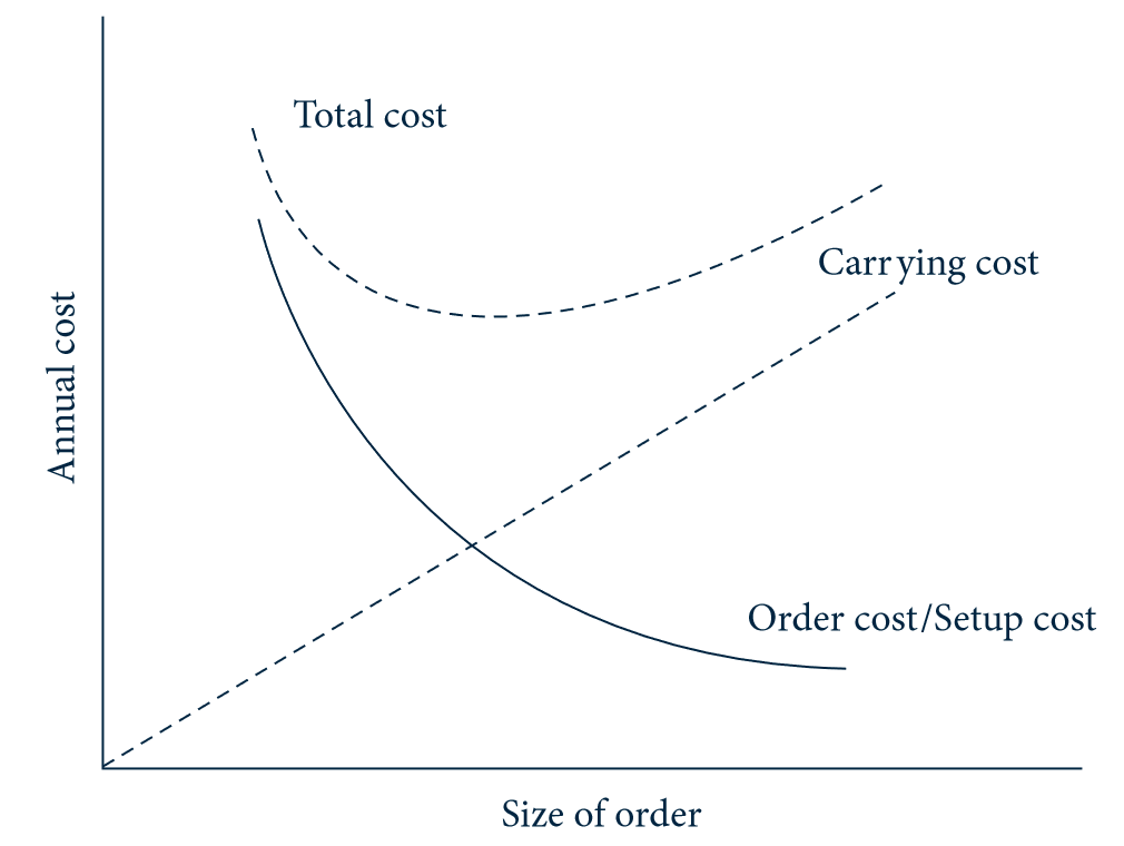
Total annual cost (TAC) equation

The total annual cost (TAC) is:

\[ TAC = \overbrace{\frac{1}{2}QVW}^{\substack{\text{Carrying}\\\text{costs}}} + \overbrace{A\frac{R}{Q}}^{\substack{\text{Ordering}\\\text{costs}}} \]

Where:

• \(Q\) = order quantity (units)
• \(R\) = annual rate of demand (units)
• \(V\) = cost of one unit of inventory
• \(W\) = carrying cost/unit of inventory/year (%)
• \(A\) = cost of placing an order

Total annual cost adds two opposing terms. Cycle-stock carrying cost is average inventory, \(Q/2\), times unit value \(V\) and annual carrying-rate \(W\). Ordering cost is cost per order \(A\) times the number of orders per year, \(R/Q\).

“Given these variables, the total annual cost for a specific economic order quantity can be expressed as either Formula 9.3 or Formula 9.4.”

\[TAC = \frac{1}{2}QVW + A\frac{R}{Q}\]

“The first term on the right-hand side of the equation refers to annual inventory carrying cost; it states that these costs equal the average number of units in the economic order quantity during the order cycle (\(\frac{1}{2}Q\)) multiplied by the value per unit (\(V\)) multiplied by the carrying cost percentage (\(W\)).”

“The second terms in Formulas 9.3 and 9.4 refer to annual ordering cost. Again, the cost to place an order is assumed to be constant, regardless of how much is ordered. Therefore, if \(Q\) increases, the number of orders placed per year will decrease since annual demand is known and constant. Larger order quantities, then, will reduce annual ordering costs.”

— Supply Chain Management: A Logistics Perspective (Coyle et al. 2020, 318–19, formulas 9.3–9.4).

EOQ graphical representation

(a) Sawtooth model

(b) Inventory carrying costs

Figure 2: Total annual costs for EOQ (Coyle et al. 2020) {#fig-tac_eoq}

The left figure explains inventory within one order cycle; the right figure explains the annual cost tradeoff. In the sawtooth model, a replenishment of \(Q\) units arrives at the start of a cycle, inventory then depletes over cycle time \(t\), and average inventory is \(Q/2\). Larger order quantities therefore raise carrying cost but reduce the number of annual orders and ordering cost.

“The first term on the right-hand side of the equation refers to annual inventory carrying cost; it states that these costs equal the average number of units in the economic order quantity during the order cycle (\(\frac{1}{2}Q\)) multiplied by the value per unit (\(V\)) multiplied by the carrying cost percentage (\(W\)). In Figure 9.9, called the sawtooth model, the equation’s logic becomes more apparent. The vertical line labeled \(Q\) represents the amount ordered at a given time and the amount of inventory on hand at the beginning of each order cycle. During the order cycle (\(t\)), an organization depletes the amount of inventory on hand at a known and constant rate (represented by the slanted line). The average number of units on hand during the order cycle is simply one-half of the economic order quantity (\(Q\)). The broken horizontal line in Figure 9.9 represents average inventory. The logic is very simple. Assuming that \(Q\) equals 100 units and that daily demand is 10 units, 100 units would last 10 days (\(t\)). At the period’s midpoint, the end of the fifth day, 50 units would still be left, which is one-half of \(Q\). Another way to examine this is to assume that average inventory during a period is beginning inventory minus ending inventory divided by 2. Since the beginning inventory equals 100 units and the ending inventory equals zero units, 100 minus zero divided by 2 results in 50 units of average inventory.”

— Supply Chain Management: A Logistics Perspective (Coyle et al. 2020, 319, fig. 9.9).

“Given the assumptions listed, the simple EOQ model considers only two basic types of cost: inventory carrying cost and ordering cost. The simple model arrives at an optimum decision that analyzes the tradeoffs between these two costs. If the model focused only on inventory carrying cost, which varies directly with changes in order quantity, the order quantity would be as small as possible (see Figure 9.6). If the model considered only ordering cost, large orders would decrease total order costs, and small orders would increase total order costs (see Figure 9.7). The lot size decision attempts to minimize total cost by reaching a compromise between these two costs (see Figure 9.8).”

“The larger the \(Q\) is, the higher the inventory carrying cost will be. This relationship was described earlier: as the order size increases, inventory carrying costs increase. Given constant demand, average inventory will increase as the economic order quantity increases.”

— Supply Chain Management: A Logistics Perspective (Coyle et al. 2020, 317–19, figs. 9.6–9.10).

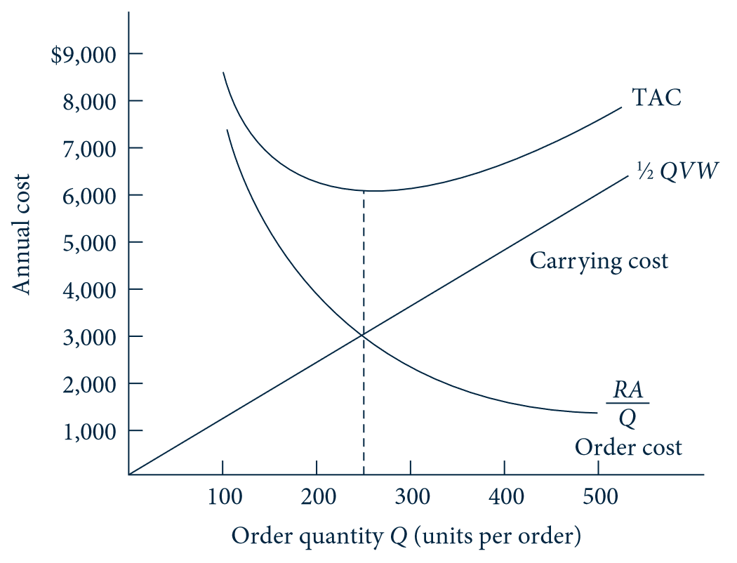
EOQ variables and total annual cost

Table 2: EOQ variables

Symbol	Description
\(R\)	Annual rate of demand (units)
\(Q\)	Quantity ordered (units)
\(\frac{1}{2}Q\)	Avg. number of units during order cycle
\(A\)	Cost of placing an order
\(V\)	Cost of one unit of inventory
\(W\)	Carrying cost/unit of inventory/year (%)
\(S\)	= \(VW\). Inventory carrying cost per unit per year
\(t\)	Order cycle time (days)
\(TAC\)	Total annual cost

The total annual cost balances inventory carrying and ordering costs:

\[ TAC = \overbrace{\frac{1}{2}QVW}^{\substack{\text{Carrying}\\\text{costs}}} + \overbrace{A\frac{R}{Q}}^{\substack{\text{Ordering}\\\text{costs}}} \]

The first term on the right-hand side of the equation refers to annual inventory carrying cost; it states that these costs equal the average number of units in the economic order quantity during the order cycle (½Q) multiplied by the value per unit (V) multiplied by the carrying cost percentage (W). In Figure 9.9, called the sawtooth model, the equation’s logic becomes more apparent. The vertical line labeled Q represents the amount ordered at a given time and the amount of inventory on hand at the beginning of each order cycle. During the order cycle (t), an organization depletes the amount of inventory on hand at a known and constant rate (represented by the slanted line). The average number of units on hand during the order cycle is simply one-half of the economic order quantity (Q). The broken horizontal line in Figure 9.9 represents average inventory. The logic is very simple. Assuming that Q equals 100 units and that daily demand is 10 units, 100 units would last 10 days (t). At the period’s midpoint, the end of the fifth day, 50 units would still be left, which is one-half of Q ( 100) 12 3 . Another way to examine this is to assume that average inventory during a period is beginning inventory minus ending inventory divided by 2. Since the beginning inventory equals 100 units and the ending inventory equals zero units, 100 minus zero divided by 2 results in 50 units of average inventory.

— Supply Chain Management: A Logistics Perspective (Coyle et al. 2020, 317).

Mathematical formulation

You may need to place an order when your current inventory levels drop below a certain level, in which case the current inventory level is the trigger for your inventory policy. Or you may want to order inventory on a set schedule, such as once a week, in which case your inventory policy is built on periodic orders. Triggering orders based on inventory levels is usually more efficient than periodic orders. But suppliers often schedule deliveries periodically because it is more convenient for them. So you need to understand the dynamics of a particular supply chain to make the best decision about which inventory trigger to use.

“The items that are managed by an inventory policy are called stock-keeping units, or SKUs (rhymes with cues). Suppose that your distribution center handles the same brand of toothpaste in three different sizes. Each size is a separate SKU.”

— Supply Chain Management For Dummies (Stanton 2023, 122).

The next question is how much to order. A mathematically precise approach to calculating your lot size is called the economic order quantity (EOQ). The EOQ formula balances the cost of placing an order against the cost of holding inventory. This formula works well on paper but usually needs to be tweaked to work in the real world. You might calculate that your EOQ is 15 widgets but discover that widgets actually come in packages of 20, for example. You also need to consider other factors when deciding how much to order, such as when a big promotion is coming up and whether you expect to have increases or decreases in demand for a product.

You can find many articles in business and engineering journals about how to calculate the EOQ, and how to modify the formula based on the unique characteristics of your supply chain.”

— Supply Chain Management For Dummies (Stanton 2023, 122).

Economic order quantity

Deriving the optimal EOQ

To find the optimal \(Q\):

1. Differentiate the \(TAC\) function: \[ \frac{\partial(TAC)}{\partial Q} = \frac{VW}{2} - \frac{AR}{Q^2 } \]
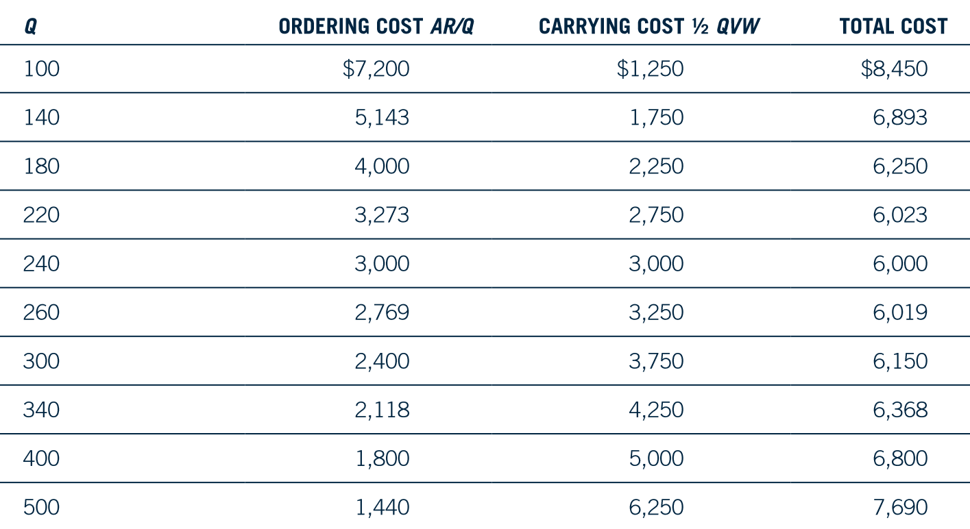
2. Set \(\frac{\partial(TAC)}{\partial Q}=0\) and solve for \(Q\): \[ \begin{align} Q^2 & = \frac{2AR}{VW} \\ Q & = \sqrt{\frac{2AR}{VW}} = \sqrt{\frac{2AR}{S}} \end{align} \]

The optimal \(Q\) is the stationary point of total annual cost. Differentiation makes the opposing rates explicit: carrying cost adds \(VW/2\) per unit increase in \(Q\), while ordering cost falls at rate \(AR/Q^2\). Setting the derivative to zero and solving yields the square-root rule.

“The discussion so far has focused on the general nature of annual inventory cost and annual ordering cost. The next step is to discuss the calculation of \(Q\), the economic order quantity. As indicated previously, this involves a tradeoff between inventory carrying cost and ordering cost. Determining \(Q\) can be accomplished by differentiating the \(TAC\) function with respect to \(Q\), as shown in Formula 9.5.”

\[\frac{d(TAC)}{dQ}=\frac{VW}{2}-\frac{AR}{Q^2}\]

“Setting \(d(TAC)/dQ\) equal to zero and solving for \(Q\) gives:”

\[Q=\sqrt{\frac{2RA}{VW}}=\sqrt{\frac{2RA}{S}}\]

“The following example illustrates how Formula 9.5 works: \(V=\$100\) per unit; \(W=25\%\); \(S=\$25\) per unit per year; \(A=\$200\) per order; \(R=3,600\) units.”

— Supply Chain Management: A Logistics Perspective (Coyle et al. 2020, 319–21, formulas 9.5–9.6).

Example

(a) Order size Q=700

(b) Order size Q=1,400

Figure 3: Sawtooth models with different order sizes and constant annual demand. As EOQ increases, inventory carrying costs and average inventory increase (Coyle et al. 2020)

The first term on the right-hand side of the total annual cost equation refers to annual inventory carrying cost. These costs equal the average number of units in the economic order quantity during the order cycle, one-half of \(Q\), multiplied by the value per unit and the carrying-cost percentage. In the sawtooth model, the vertical line labeled \(Q\) represents the amount ordered and the inventory on hand at the beginning of each order cycle. During the cycle, the organization depletes inventory at a known and constant rate. The average number of units on hand during the order cycle is one-half of the economic order quantity. For example, if \(Q\) equals 100 units and daily demand is 10 units, the order lasts 10 days. At the period’s midpoint, 50 units remain, which is one-half of \(Q\).

Determining the average number of units is only part of the equation. The value per unit and the percentage carrying cost are also necessary. The larger \(Q\) is, the higher the inventory carrying cost will be. Given constant demand, average inventory increases as the economic order quantity increases, as the two sawtooth models illustrate.

The annual ordering-cost term behaves in the opposite direction. The cost to place an order is assumed to be constant regardless of how much is ordered. Therefore, if \(Q\) increases, the number of orders placed per year decreases because annual demand is known and constant. Larger order quantities reduce annual ordering costs. The economic order quantity is determined by balancing this decrease in ordering cost against the increase in inventory carrying cost.

— Supply Chain Management: A Logistics Perspective (Coyle et al. 2020, 347–48).

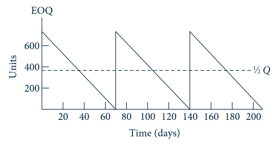
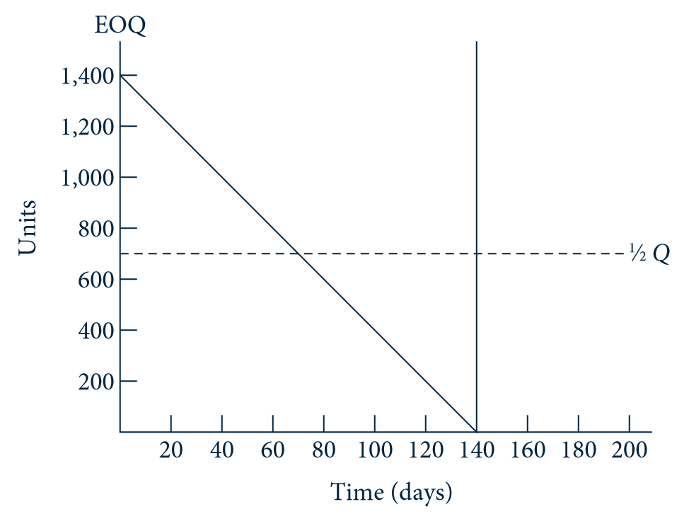
EOQ example

(a) Total cost for various EOQ amounts. Lower Q quantities result in higher annual ordering costs but lower inventory carrying costs

(b) EOQ can be changed considerably without significantly affecting TAC (shallow curve in range 180–320)

Figure 4: The optimal Q is 240 units considering \(V\) = $100 per unit, \(W\) = 25%, \(S\) = $25 per unit per year, \(A\) = $200 per order, and \(R\) = 3,600 units (Coyle et al. 2020)

V = $100 per unit - W = 25% - S = $25 per unit per year - A = $200 per order - R = 3,600 units Analysis Table 9.13 and Figure 9.11 show the proceeding solution’s tradeoffs and logic. These illustrations show how inventory carrying cost, ordering cost, and total cost vary as Q ranges from a low of 100 units to a high of 500 units. As Table 9.13 shows, the lower quantities of Q result in higher annual ordering costs but result in lower annual inventory carrying costs, as expected. As Q increases from 100 to 240 units, annual ordering costs decrease because the number of orders placed per year decreases while annual inventory carrying costs increase because of the higher average inventories. Beyond 240 units, the incremental increase in annual inventory carrying cost exceeds the incremental decrease in annual ordering cost, thereby increasing total annual cost. By defining the optimum Q in total cost terms, the data in Table 9.13 show that a Q of 240 units is optimal (least total cost). Figure 9.11 also demonstrates this optimum level. Note, however, that the TAC curve between EOQ values of 180 to 200 units and 300 to 320 units is quite shallow. This means that the inventory manager can alter the EOQ considerably without significantly affecting TAC. Using the previous example, assume that order transmittal takes one day, order processing and preparation take two days, and order delivery takes five days. This results in a replenishment or lead time of eight days. Given that demand is 10 units per day (3,600 units/360 days), the reorder point will be 80 units (8 days × 10 units per day).

— Supply Chain Management: A Logistics Perspective (Coyle et al. 2020, 349).

— Supply Chain Management: A Logistics Perspective (Coyle et al. 2020, 350).

Reorder point (the “when”)

Under the assumptions of certainty, an organization needs only enough inventory to last during the replenishment time or lead time.

Replenishment time consists of:

• order transmittal (electronic, manual)
• order processing (inventory availability)

• order preparation
• order delivery (transportation mode)

Given a lead time, we have:

\[ \text{Reorder point} = \text{Lead time} \times \text{daily demand} \]

Example:

• \(\text{Lead time}\) = 1 day (transmittal) + 2 days (processing & preparation) + 5 days (delivery) = 8 days.
• \(\text{Daily demand}\) = 10 units/day (3,600 units/360 days).
• \(\text{Reorder point}\) = 8 days × 10 units/day = 80 units.

Therefore, given a known lead time, multiplying lead time length by daily demand determines the reorder point. Reorder Point A previous discussion indicated that knowing when to order was as necessary as knowing how much to order. The when, called the reorder point, depends on the inventory level on hand. Under the assumptions of certainty, an organization needs only enough inventory to last during the replenishment time or lead time. Therefore, given a known lead time, multiplying lead time length by daily demand determines the reorder point. Replenishment time consists of several components: order transmittal, order processing, order preparation, and order delivery. The time for each depends on factors such as the means used to transmit the order (electronic versus manual), the inventory availability at the supplier, and the transportation mode used for delivery. Factors affecting lead time will be discussed later in this chapter. Using the previous example, assume that order transmittal takes one day, order processing and preparation take two days, and order delivery takes five days. This results in a replenishment or lead time of eight days. Given that demand is 10 units per day (3,600 units/360 days), the reorder point will be 80 units (8 days × 10 units per day).

— Supply Chain Management: A Logistics Perspective (Coyle et al. 2020, 349).

Summary

• Useful to illustrate the logic of inventory management.
• Not the fastest way to respond to customer demand.
• Can be adjusted to handle more complex situations.
  • Organizations adapt EOQ-based approaches to include push/pull orientation.
  • Push (proactive inventory management) approaches are more prevalent in organizations having greater logistics sophistication.
• Suits inventory decision-making at a single facility.
• Not robust to simultaneous demand peaks (e.g., many customers stocking up on groceries).

“Summary and Evaluation of the Fixed Order Quantity Approach Traditionally, the EOQ approach has been a cornerstone of effective inventory management. While not always the fastest way to respond to customer demand, the fixed order quantity approach has been a widely used technique. Recently, however, many organizations have become more sophisticated in their use of EOQ-based approaches, adapting them to include a push as well as a pull orientation. As a result, many EOQ-based systems effectively blend both push and pull concepts. As indicated earlier, push, or proactive, inventory management approaches are far more prevalent in organizations having greater logistics sophistication.

One principal shortcoming of the EOQ-based approach is that it suits inventory decision making at a single facility more than it suits decision making at multiple locations in a logistics network. Also, the EOQ approach sometimes encounters problems when parallel points in the same logistics system experience peak demands simultaneously. This happens, for example, when many consumers simultaneously stock up on groceries before a major snowstorm. The EOQ approach alone, reacting to demand levels only as they occur, would respond too slowly to replenish needed inventory. As stated at the outset, the simple EOQ approach, though somewhat unrealistic because of the number of assumptions it requires, is still useful because it illustrates the logic of inventory models in general.

Actually, organizations can adjust the simple model to handle more complex situations. Appendix 9A covers applications of the EOQ approach in four special instances: (1) when an organization must consider the cost of inventory in transit, (2) when volume transportation rates are available, (3) when an organization uses private transportation, and (4) when an organization utilizes in-excess freight rates.

Typically, organizations associate EOQ-based approaches with independent, rather than dependent, demand. However, the EOQ approach can also be used for dependent demand items. The overall approach explicitly involves carrying calculated average inventory amounts; the tradeoffs among inventory, order, and expected stockout costs justify carrying these amounts.”

— Supply Chain Management: A Logistics Perspective (Coyle et al. 2020, 323).

Summary

Warehouse storage optimization: Reorder point under uncertainty

01

Fixed order quantity approach (condition of uncertainty)

Most organizations do not operate under conditions of certainty:

• Demand rates depend on many factors, such as:
  • weather and sporadic social or physical needs;
  • day, week, and season.
• Lead times depend on (long-distance) transit times.
  • Transit times:
    • Affected by many factors, such as: weather, highway congestion, port congestion, border stops.
  • Order transmittal and processing (e.g., credit blocks, inventory unavailability).

“9-5d Fixed Order Quantity Approach (Condition of Uncertainty)

Under the assumptions used until now, the reorder point was based on the amount of inventory on hand and demand was known and constant. When inventory on hand reached zero, a new order was received in an economic order quantity and stockout costs were not incurred. Although assuming such conditions of certainty might be useful to simplify inventory models, these conditions do not represent the normal situations faced by most organizations today.

Most organizations would not operate under conditions of certainty for a variety of reasons. First, consumers usually purchase products somewhat sporadically. The demand rates for many products vary depending on weather, social needs, physical needs, and a whole host of other factors. As a result, the demand for most products varies by day, week, and season. In addition, several factors can affect lead time. For example, transit times can and do change, particularly over long distances, despite transportation provider efforts. Factors such as weather, highway congestion, port congestion, and border stops can make transit times very unreliable. In fact, transit time reliability is a major factor used by organizations when they are making both mode and carrier decisions. Other factors that can cause variations in lead time are order transmittal and processing. Although a significant number of orders today are transmitted electronically, many are still sent through the U.S. Post Office. Mailed orders can be subject to the same unreliability in transit time as mentioned previously. During order processing, factors such as credit blocks and inventory unavailability can cause delays in orders proceeding through the system.

Because of all the potential factors that can influence the reliability of demand and lead time, inventory models need to be adjusted to account for this uncertainty.

”

— Supply Chain Management: A Logistics Perspective (Coyle et al. 2020, 323).

Adjusting inventory models to account for uncertainty

Figure 5: Fixed order quantity model adjusted for uncertainty. Uncertain demand and lead time may lead to stockouts and excess inventory (Coyle et al. 2020)

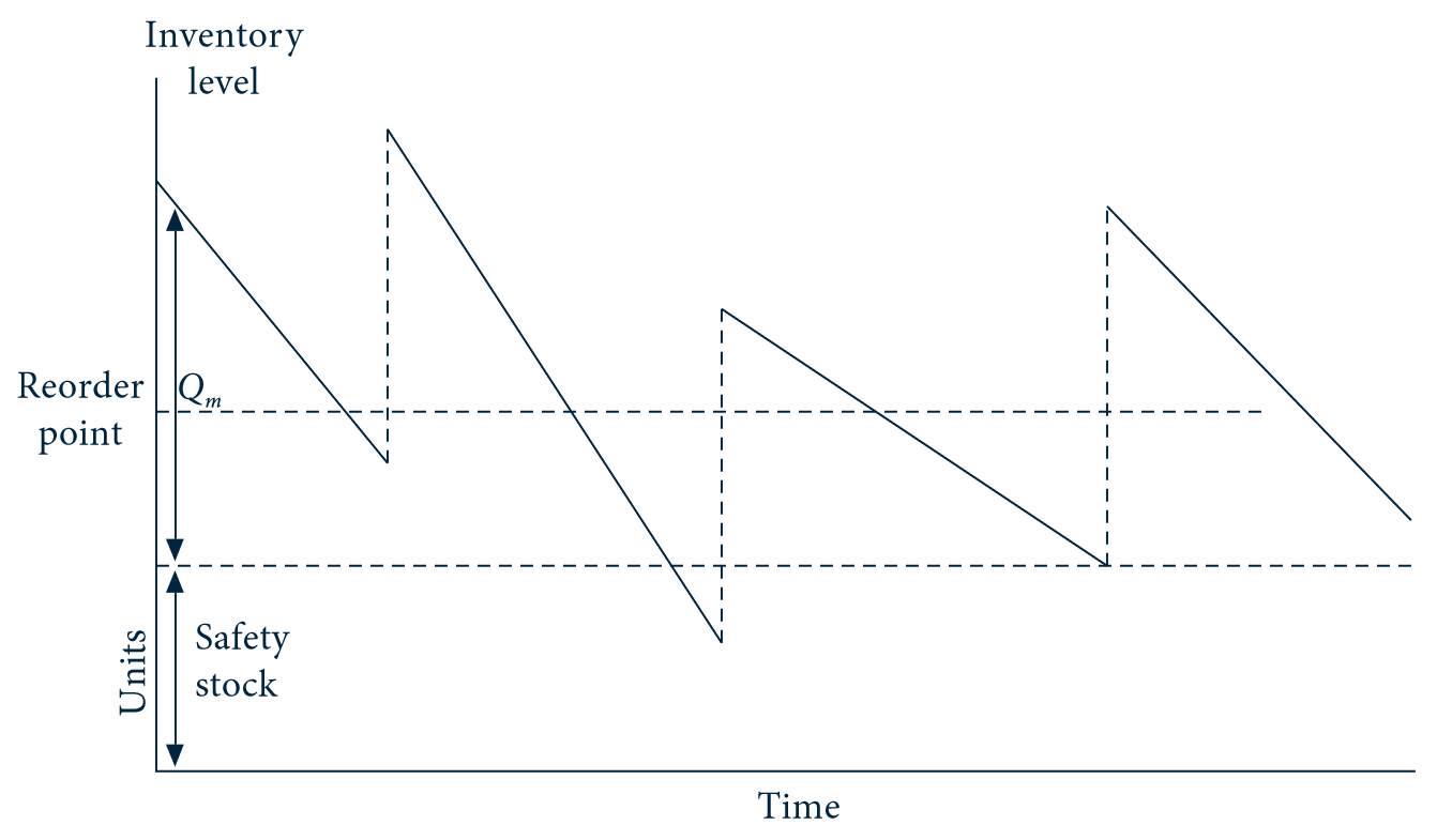
• Demand
  • Not known or constant.
  • Result: on-hand inventory line fluctuates
    • above the EOQ amount;
    • below zero units.
• Lead time (or cycle)
  • Not known or constant.
  • Result: varying period length.
• Safety stock
  • Amount depends on
    • demand/lead time variability;
    • customer service requirements.

Figure 9.12 shows the fixed order quantity model adjusted for uncertainty in demand and lead time. This figure varies from the model introduced in Figure 9.5 in three ways. First, demand (affecting on-hand inventory levels) in Figure 9.5 was known and constant. This is why the on-hand inventory line in Figure 9.5 always begins the period at the EOQ amount and ends the period at zero units. This same line in Figure 9.12 fluctuates above the EOQ amount and below zero units because demand is not known or constant. Second, the lead time (or cycle) in Figure 9.5 is known and constant at five weeks, resulting in a very uniform “sawtooth” pattern. When lead time is not known or constant, as shown in Figure 9.12, the length of the period (or lead time) varies resulting in an uneven spacing between orders. Finally, Figure 9.5 makes no allowances for stockouts since its assumptions present conditions of certainty. In Figure 9.12, the uncertainty of demand and lead time makes necessary the addition of safety stock to prevent stockouts. The amount of safety stock to be held will depend on the variability around demand and lead time and the service customers require.”

— Supply Chain Management: A Logistics Perspective (Coyle et al. 2020, 352).

Safety stock

• A tradeoff exists between the cost of holding safety stock versus the cost of a stockout.
• Many techniques exist for setting safety stock levels (see King 2011).
• As service level requirements increase, safety stocks increase at an increasing rate.

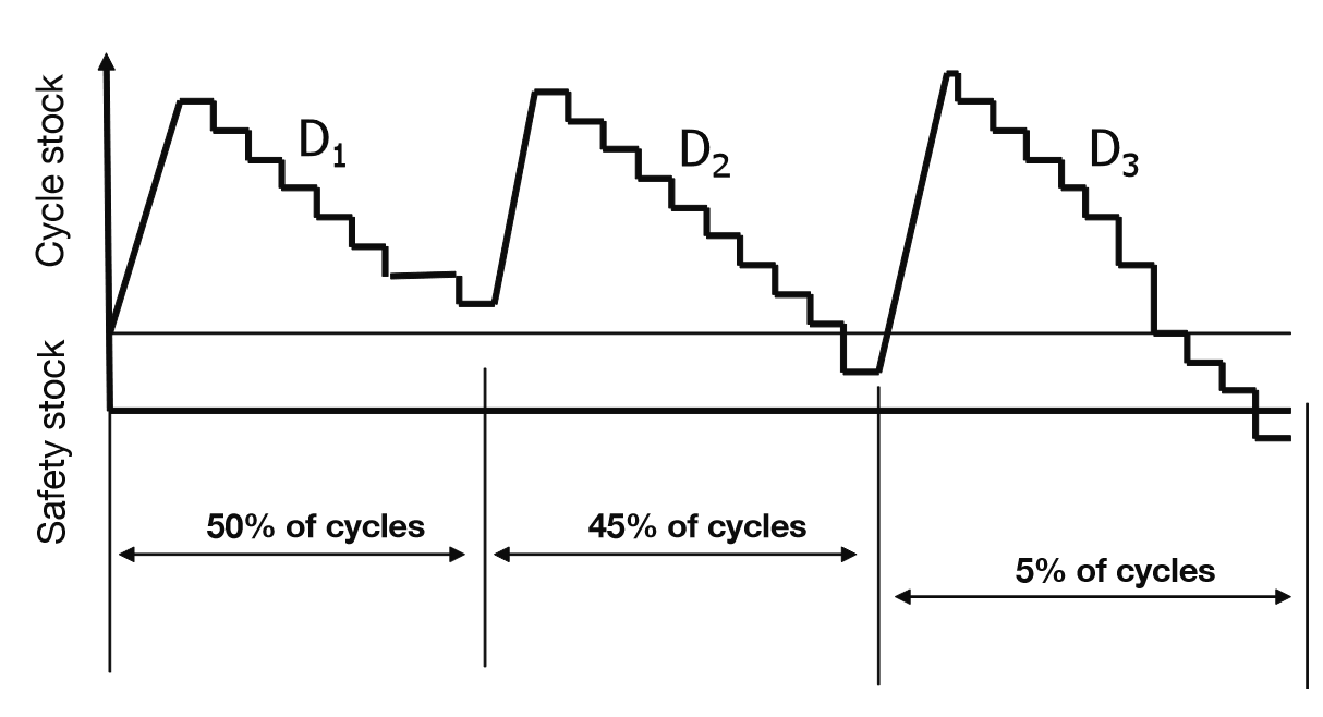
Figure 6: Inventory designed for a 95% service level (King 2011)

Safety stock is the inventory held beyond expected cycle requirements to absorb uncertainty. It reduces rather than eliminates stockouts. Raising the target service level requires progressively more protection because the service-level–Z-score relationship is nonlinear.

“Safety stock simply is inventory that is carried to prevent stockouts. Stockouts stem from factors such as fluctuating customer demand, forecast inaccuracy, and variability in lead times for raw materials or manufacturing. Some operations managers use gut feelings or hunches to set safety stock levels, while others base them on a portion of cycle stock level—10 or 20 percent, for example. While easy to execute, such techniques generally result in poor performance. A sound, mathematical approach to safety stock will not only justify the required inventory levels to business leaders, but also balance the conflicting goals of maximizing customer service and minimizing inventory cost.”

“Safety stock determinations are not intended to eliminate all stockouts—just the majority of them. For example, when designing for a 95 percent service level, expect that 50 percent of the time, not all cycle stock will be depleted and safety stock will not be needed. For another 45 percent of cycles, the safety stock will suffice. But in approximately 5 percent of replenishment cycles, expect a stockout.”

“As illustrated, the relationship is nonlinear: Higher cycle service levels require disproportionally higher Z-scores and, thus, disproportionately higher safety stock levels. Typical goals fall between 90 and 98 percent, and—statistically speaking—a cycle service level of 100 percent is unattainable.”

— Understanding Safety Stock and Mastering Its Equations (King 2011, 33–34, figs. 1–2).

Adjusting the reorder point

EOQ model with certainty

The reorder point is the on-hand inventory level needed to satisfy demand during lead time.

EOQ model under uncertainty

The reorder point is the average daily demand during lead time plus the safety stock.

“Reorder Point—A Special Note

As noted previously, the reorder point under the basic model is the on-hand inventory level needed to satisfy demand during lead time. Calculating the reorder point is relatively easy since demand and lead time are constant. Under uncertainty, an organization must reformulate the reorder point to allow for safety stock. In effect, the reorder point becomes the average daily demand during lead time plus the safety stock, as Figure 9.12 shows. The following discussion clarifies this recalculation.”

— Supply Chain Management: A Logistics Perspective (Coyle et al. 2020, 324).

Reorder point (special note)

Uncertainty of demand

How much product customers will demand during a constant/known lead time when usage rate is varying?

The reorder level must balance:

1. Cost of carrying safety stock
2. Stockout (lost sales) costs

If the reorder level is:

• Too high = too much stock on hand when the next order arrives.
• Too low = stockout leading to lost sales.

In discussing demand, logistics managers emphasize balancing the cost of carrying safety stock against the cost of a stockout (lost sales).

In a fixed quantity model with an established reorder point, introducing uncertainty into the analysis initially affects the inventory level needed to cover demand during lead time.

Recall that in the previous example, conditions of certainty resulted in an EOQ of 240 units and a reorder point of 100 units. In other words, the inventory period began with 240 units on hand, and reordering occurred when inventory reached a level of 100 units. The fact that demand will vary—and that the time that elapses between a level of 240 units and 100 units might vary—is not critical to the inventory problem when conditions of uncertainty exist. Determining whether 100 units is the best amount to have on hand at the start of the lead time cycle is critical. Thus, raising the reorder level accounts for safety stock. However, raising it too high will leave too much stock on hand when the next order arrives. Setting it too low will result in a stockout. Using the previous problem, assume that the organization’s demand during lead time ranges from 100 units to 160 units, with an average of 130 units. Also assume that demand has a discrete distribution varying in 10-unit blocks and that the organization has established probabilities for these demand levels (see Table 9.14). In effect, the organization must consider seven different reorder points, each corresponding to a possible demand level as shown in Table 9.14. Using these reorder points, the matrix in Table 9.15 can be developed.
While Table 9.15 shows many of the possible situations confronting the organization, it does not use information from the probability distribution of demand. Using the probability of demand would allow the organization with seven possible reorder points to determine the expected units short or in excess at each point during lead time. Assume that the organization incurs a stockout cost (k) of $10 per unit whenever a customer demands a unit that is not in inventory. The profit lost on the immediate sale and future sales is an opportunity cost. Inventory carrying cost associated with safety stock is calculated the same way as it was for calculating carrying cost for the simple EOQ model. The value per unit is still assumed to be $100, and the percentage annual inventory carrying cost is still 25 percent. Remember that the percentage figure is for the annual cost of inventory stored in the warehouse. Therefore, the $25 derived by multiplying 25 percent by $100 is the annual cost per unit of inventory in the warehouse. The $25 contrasts with the $10 stockout cost, which is a unit cost per cycle of order period. Therefore, as Table 9.16 shows, multiplying $10 by the number of cycles or orders per year translates this cost into an annual basis.

Table 9.16 develops expected units short or in excess by multiplying the number of units short or in excess by the probabilities associated with each demand level. The numbers below (shorts) and above (in excess) the horizontal line are added, as the lower portion of Table 9.16 shows, to find the number of units the organization expects to be short or in excess at each of the seven possible reorder points. The variables for this calculation are as follows: Expected excess in units Expected shorts in units Stockout cost in dollars perunitstocked out Expected stockout cost percycle () Expected stockout cost peryear Expected carryingcostper year forexcessinventory
After performing the calculations indicated in Table 9.16, the total cost for each of the seven reorder points may be calculated. In this instance, the lowest total cost corresponds to the reorder point of 140 units. Although this number does not guarantee an excess or a shortage in any particular period, it gives the overall lowest total cost per year: $390. Note that the number of orders used in Step 5 of Table 9.16 came from the preceding problem with conditions of certainty. This number was the only information available at that point. Now the total cost model can be expanded to include the safety stock and stockout cost. Formula 9.7 represents the expanded equation. QVWAR Q eVW R GQ TAC 1 2 () 511  1   9.7 Solving for the lowest total cost gives Formula 9.8. d dQ VW RA G Q TAC1 22 521 () ()         9.8 Setting this equal to zero and solving for Q results in Formula 9.9. 51 2( ) Q RA G VW

Using the expanded model and the computed reorder point of 140 units, a new value for Q can be calculated as shown in Formula 9.10. 5 331 3 5 2, 3600 (200 8) $100 25% 245 unitsapproximately Q 9.10 Note that Q is now 245 units with conditions of uncertainty. Technically, this would change the expected stockout cost for the various reorder points in Table 9.16. However, the change is small enough to ignore in this instance. In other cases, recalculations might be necessary. The optimum solution to the problem with conditions of uncertainty is a fixed order quantity of 245 units, and the organization will reorder this amount when inventory reaches a level of 140 units (the calculated reorder point). Finally, this situation requires a recalculation of total annual cost as shown in Formula 9.11. QVWAR Q eVWGR Q TAC 1 2 1 2 245 $100 25% 200 3,600 245 (10.8 1 $00 25%)83,600 245 $3,062.50 $2,938.78 $270 $117.55 $6,389 5111 53 33 13 13313 5111 5             9.11 The $6,389 figure indicates what happens to total annual cost when conditions of uncertainty with respect to demand are introduced into the model. Introducing other factors, such as the lead time factor, would increase costs even more.

— Supply Chain Management: A Logistics Perspective (Coyle et al. 2020, 325).

Uncertainty of demand

Assumptions:

1. A continuous, constant, and known rate of demand
2. A constant and known replenishment or lead time
3. All demand is satisfied
4. A constant price or cost that is independent of the order quantity

5. No inventory in transit
6. One item of inventory or no interaction between items
7. Infinite planning horizon
8. Unlimited capital

Example: Lowest cost reorder point calculation

Different reorder points are considered for possible demands within the lead time:

Input: Expected demand prob. distribution

Demand (units)	Prob.
100	0.01
110	0.06
120	0.24
130	0.38
140	0.24
150	0.06
160	0.01

This example replaces one certain lead-time demand value with a discrete probability distribution. Each possible demand level is also considered as a candidate reorder point, creating seven policies to compare.

Table transcription: Table 9.14 assigns probabilities 0.01, 0.06, 0.24, 0.38, 0.24, 0.06, and 0.01 to lead-time demands of 100, 110, 120, 130, 140, 150, and 160 units, respectively (Coyle et al. 2020, 325, table 9.14).

“Using the previous problem, assume that the organization’s demand during lead time ranges from 100 units to 160 units, with an average of 130 units. Also assume that demand has a discrete distribution varying in 10-unit blocks and that the organization has established probabilities for these demand levels (see Table 9.14). In effect, the organization must consider seven different reorder points, each corresponding to a possible demand level as shown in Table 9.14.”

— Supply Chain Management: A Logistics Perspective (Coyle et al. 2020, 325, table 9.14).

Step 1: Inventory shortage or excess

Possible units of inventory in shortage or excess:

Actual demand	100	110	120	130	140	150	160
100	0	10	20	30	40	50	60
110	-10	0	10	20	30	40	50
120	-20	-10	0	10	20	30	40
130	-30	-20	-10	0	10	20	30
140	-40	-30	-20	-10	0	10	20
150	-50	-40	-30	-20	-10	0	10
160	-60	-50	-40	-30	-20	-10	0

Each column is a candidate reorder point and each row is an actual lead-time demand outcome. The cell is zero when demand equals the reorder point. A positive difference above the diagonal is excess inventory; a negative difference below the diagonal is a shortage.

“In effect, the organization must consider seven different reorder points, each corresponding to a possible demand level as shown in Table 9.14. Using these reorder points, the matrix in Table 9.15 can be developed.”

“While Table 9.15 shows many of the possible situations confronting the organization, it does not use information from the probability distribution of demand. Using the probability of demand would allow the organization with seven possible reorder points to determine the expected units short or in excess at each point during lead time.”

— Supply Chain Management: A Logistics Perspective (Coyle et al. 2020, 325–26, table 9.15).

Step 2: Expected short or excess units

Expected number of units in short or in excess:

Actual demand	Prob.	100	110	120	130	140	150	160
100	0.01	0.0	0.1	0.2	0.3	0.4	0.5	0.6
110	0.06	-0.6	0.0	0.6	1.2	1.8	2.4	3
120	0.24	-4.8	-2.4	0.0	2.4	4.8	7.2	9.6
130	0.38	-11.4	-7.6	-3.8	0.0	3.8	7.6	11.4
140	0.24	-9.6	-7.2	-4.8	-2.4	0.0	2.4	4.8
150	0.06	-3.0	-2.4	-1.8	-1.2	-0.6	0.0	0.6
160	0.01	-0.6	-0.5	-0.4	-0.3	-0.2	-0.1	0.0

The matrix becomes decision-relevant only after weighting every shortage or excess by the probability of its demand outcome. For each candidate reorder point, the weighted excess cells and weighted shortage cells are summed separately to obtain expected excess \(e\) and expected shortage \(g\) per cycle.

The notation is a normalized glossary of Table 9.16: \(e\) is expected excess in units; \(g\) is expected shorts in units; \(k\) is stockout cost per unit stocked out; \(G=gk\) is expected stockout cost per cycle; \(G(R/Q)\) is expected stockout cost per year; and \(eVW\) is expected annual carrying cost for excess inventory (Coyle et al. 2020, 326–27, table 9.16).

“Table 9.16 develops expected units short or in excess by multiplying the number of units short or in excess by the probabilities associated with each demand level. The numbers below (shorts) and above (in excess) the horizontal line are added, as the lower portion of Table 9.16 shows, to find the number of units the organization expects to be short or in excess at each of the seven possible reorder points.”

— Supply Chain Management: A Logistics Perspective (Coyle et al. 2020, 326–27, table 9.16).

Inputs for annual cost evaluation

Input: EOQ variables

• Annual demand (\(R\)) = 3,600 units/year
• Demand within lead time = 100–160 units
• EOQ (\(Q\)) = 240 units (estimated before)
• Stockout cost (\(k\)) = $10
• Carrying cost/unit/year (\(W\)) = 25%
• Cost of one unit of inventory (\(V\)) = $100
• Carrying cost/year (\(VW\)) = $25
• Avg. demand = 130

These inputs combine the earlier certainty example with the uncertainty extension. The $10 stockout cost is per unit short in one replenishment cycle; multiplying expected cost per cycle by \(R/Q\), the expected annual number of orders, converts it to an annual cost.

“The following example illustrates how Formula 9.5 works:”

• \(V = \$100\) per unit
• \(W = 25\%\)
• \(S = \$25\) per unit per year
• \(A = \$200\) per order
• \(R = 3,600\) units

“To solve for \(Q\), the example proceeds as shown in Formula 9.6.”

\[Q=\sqrt{\frac{2RA}{VW}}=\sqrt{\frac{(2)(3,600)(\$200)}{(\$100)(25\%)}}=240\text{ units}\]

— Supply Chain Management: A Logistics Perspective (Coyle et al. 2020, 320–21, formulas 9.5–9.6).

“Using the previous problem, assume that the organization’s demand during lead time ranges from 100 units to 160 units, with an average of 130 units. Also assume that demand has a discrete distribution varying in 10-unit blocks and that the organization has established probabilities for these demand levels (see Table 9.14).”

— Supply Chain Management: A Logistics Perspective (Coyle et al. 2020, 325, table 9.14).

“Assume that the organization incurs a stockout cost (\(k\)) of $10 per unit whenever a customer demands a unit that is not in inventory. The profit lost on the immediate sale and future sales is an opportunity cost.”

“Inventory carrying cost associated with safety stock is calculated the same way as it was for calculating carrying cost for the simple EOQ model. The value per unit is still assumed to be $100, and the percentage annual inventory carrying cost is still 25 percent. Remember that the percentage figure is for the annual cost of inventory stored in the warehouse. Therefore, the $25 derived by multiplying 25 percent by $100 is the annual cost per unit of inventory in the warehouse. The $25 contrasts with the $10 stockout cost, which is a unit cost per cycle of order period. Therefore, as Table 9.16 shows, multiplying $10 by the number of cycles or orders per year translates this cost into an annual basis.”

— Supply Chain Management: A Logistics Perspective (Coyle et al. 2020, 326–27, table 9.16).

Step 3: Lowest-cost reorder point

The lowest-cost reorder point minimizes annual stockout and carrying costs:

Calculation of lowest cost reorder point	100	110	120	130	140	150	160
1. Expected excess/cycle (\(e\))	0	0.1	0.8	3.9	10.8	20.1	30
2. Expected carrying cost/year (\(eVW\))	$0	$2.50	$20.00	$97.50	$270	$502.50	$750
3. Expected shorts/cycle (\(g\))	30	20.1	10.8	3.9	0.8	0.1	0
4. Expected stockout cost/cycle (\(gk\)) = \(G\)	$300	$201	$108	$39	$8	$1	$0
5. Expected stockout cost/year (\(G\frac{R}{Q}\))	$4,500	$3,015	$1,620	$585	$120	$15	$0
6. Expected total cost/year (2. + 5.)	$4,500	$3,017.50	$1,640	$682.50	$390	$517.50	$750

For each candidate reorder point, Table 9.16 adds annual carrying cost for expected excess stock to annual expected stockout cost. The best policy is the least-cost column, not a promise that every cycle will avoid excess or shortage.

“After performing the calculations indicated in Table 9.16, the total cost for each of the seven reorder points may be calculated. In this instance, the lowest total cost corresponds to the reorder point of 140 units. Although this number does not guarantee an excess or a shortage in any particular period, it gives the overall lowest total cost per year: $390.”

“Note that the number of orders used in Step 5 of Table 9.16 came from the preceding problem with conditions of certainty. This number was the only information available at that point. Now the total cost model can be expanded to include the safety stock and stockout cost.”

— Supply Chain Management: A Logistics Perspective (Coyle et al. 2020, 327, table 9.16).

Optimal EOQ notation

Table 3: EOQ variables

Symbol	Description
\(R\)	Annual rate of demand (units)
\(Q\)	Quantity ordered (units)
\(\frac{1}{2}Q\)	Avg. number of units during order cycle
\(A\)	Cost of placing an order
\(V\)	Cost of one unit of inventory
\(W\)	Carrying cost/unit of inventory/year (%)
\(e\)	Expected excess in units
\(g\)	Expected shorts in units
\(k\)	Stockout cost in dollars per unit stocked out
\(G=gk\)	Expected stockout cost per cycle
\(G\frac{R}{Q}\)	Expected stockout cost per year
\(eVW\)	Expected carrying cost per year for excess inventory

“Therefore, probability theory informs us that, when lead time and demand are uncorrelated, the standard deviation of total demand in a lead time is (Feller 1957).”

— Safety Stock Determination Based on Parametric Lead Time and Demand Information (Lisan 2018, 4).

shows these figures and the ones computed for setting the reorder point at two and three standard deviations from the mean. An organization should thoroughly compare the financial and customer service benefits of avoiding stockouts with the cost of carrying additional safety stock before choosing a reorder point.

Uncertainty of Demand and Lead Time Length

This section considers the possibility that both demand and lead time might vary and builds on the preceding section in attempting to make this inventory approach more realistic. As expected, however, determining how much safety stock to carry will be noticeably more complex now than when only demand varied (the mathematical determination of safety stock when both demand and lead time vary was covered at the beginning of this chapter). As in the previous section, the critical issue is just how much product customers will demand during the lead time. If demand and lead time are constant and known, calculating the reorder point (as was done in the section covering the case of certainty) would be easy. Now that both demand and lead time might vary, the first step is to identify the likely distribution of demand during the lead time. Specifically, the mean and standard deviation of demand during lead time must be estimated. Figure 9.13 illustrates two key properties of a normal distribution. These concepts were covered earlier in this chapter, but it is important to revisit them here in the context of the fixed order quantity model under uncertainty. First, the normal distribution is symmetrical, with approximately 68.26 percent of all observations within one standard deviation around the mean, 95.44 percent within two standard deviations, and 99.73 percent within three standard deviations. Second, in the normal distribution, the mode (highest point or most observations) equals the mean (average). After calculating values for the mean and standard deviation of demand during lead time, the stockout probability for each particular reorder point can be described. For example, assume that Figure 9.13 represents the demand distribution during lead time. Setting the reorder point equal to X- + 1σ will result in an 84.13 percent probability that lead time demand will not exceed the inventory amount available. Increasing the reorder point to X- + 2σ raises the probability of not incurring a stockout to 97.72 percent; reordering at X- + 3σ raises this probability to 99.87 percent.

Note that in the case of uncertainty, increasing the reorder point has the same effect as increasing the safety stock commitment. An organization must ultimately find some means to justify carrying this additional inventory.

Borrowing Formula 9.1, the mean and standard deviation for demand during lead time can be calculated as shown in Formulas 9.12 and 9.13. 5 X SR 9.12 s5 s1s () () 22 2 RS SR where: X R S R S Averagedemandduringleadtime(units) Standard deviationofdemandduringleadtime(units) Averagereplenishment cycle(days) Standard deviationofreplenishmentcycle(days) Averagedaily demand (units) Standard deviationofdaily demand (units) 5 s5 5 s5 5 s5 For example, if the mean and standard deviation of daily demand are 20 and four units, respectively, and if the mean and standard deviation of lead time are eight and two days, respectively, then the mean and standard deviation of demand during lead time can be calculated as shown in Formula 9.14. 5 5 5 20(8) 160units XR S 9.14 s5 s1s 51 5 5 RS () () (8)(4) (20) (2) 1, 728 41.57 or 42 units SR 222 222 Using the procedure suggested earlier, setting the reorder point at X 1 1σ, or 202 units, reveals an 84.13 percent probability that demand during lead time will not exceed the inventory available. Stated differently, the probability of a stockout is only 15.87 percent (100% 2 84.13%) when the reorder point is set at one standard deviation from the mean. Table 9.17 shows these figures and the ones computed for setting the reorder point at two and three standard deviations from the mean. An organization should thoroughly compare the financial and customer service benefits of avoiding stockouts with the cost of carrying additional safety stock before choosing a reorder point.

— Supply Chain Management: A Logistics Perspective (Coyle et al. 2020, 356).

Table:

— Supply Chain Management: A Logistics Perspective (Coyle et al. 2020, 358).

Optimal EOQ mathematical formulation

To find the optimal \(Q\):

1. Calculate the total annual cost: \[ \begin{align} TAC = \overbrace{\frac{1}{2}QVW}^{\substack{\text{Carrying}\\\text{costs}}} + \overbrace{A\frac{R}{Q}}^{\substack{\text{Ordering}\\\text{costs}}} + \overbrace{(eVW)}^{\substack{\text{Safety}\\\text{cost}}} + \overbrace{\left(G\frac{R}{Q}\right)}^{\substack{\text{Stockout}\\\text{cost}}} \end{align} \]

2. Differentiate the \(TAC\) function: \[ \begin{align} \frac{\partial(TAC)}{\partial Q} = \frac{1}{2}VW - \frac{R(A+G)}{Q^2} \end{align} \]

3. Set \(\frac{\partial(TAC)}{\partial Q}=0\) and solve for \(Q\): \[ \begin{align} Q & = \sqrt{\frac{2R(A+G)}{VW}} \end{align} \]

“Therefore, probability theory informs us that, when lead time and demand are uncorrelated, the standard deviation of total demand in a lead time is (Feller 1957).”

— Safety Stock Determination Based on Parametric Lead Time and Demand Information (Lisan 2018, 4).

shows these figures and the ones computed for setting the reorder point at two and three standard deviations from the mean. An organization should thoroughly compare the financial and customer service benefits of avoiding stockouts with the cost of carrying additional safety stock before choosing a reorder point.

Uncertainty of Demand and Lead Time Length

This section considers the possibility that both demand and lead time might vary and builds on the preceding section in attempting to make this inventory approach more realistic. As expected, however, determining how much safety stock to carry will be noticeably more complex now than when only demand varied (the mathematical determination of safety stock when both demand and lead time vary was covered at the beginning of this chapter). As in the previous section, the critical issue is just how much product customers will demand during the lead time. If demand and lead time are constant and known, calculating the reorder point (as was done in the section covering the case of certainty) would be easy. Now that both demand and lead time might vary, the first step is to identify the likely distribution of demand during the lead time. Specifically, the mean and standard deviation of demand during lead time must be estimated. Figure 9.13 illustrates two key properties of a normal distribution. These concepts were covered earlier in this chapter, but it is important to revisit them here in the context of the fixed order quantity model under uncertainty. First, the normal distribution is symmetrical, with approximately 68.26 percent of all observations within one standard deviation around the mean, 95.44 percent within two standard deviations, and 99.73 percent within three standard deviations. Second, in the normal distribution, the mode (highest point or most observations) equals the mean (average). After calculating values for the mean and standard deviation of demand during lead time, the stockout probability for each particular reorder point can be described. For example, assume that Figure 9.13 represents the demand distribution during lead time. Setting the reorder point equal to X- + 1σ will result in an 84.13 percent probability that lead time demand will not exceed the inventory amount available. Increasing the reorder point to X- + 2σ raises the probability of not incurring a stockout to 97.72 percent; reordering at X- + 3σ raises this probability to 99.87 percent.

Note that in the case of uncertainty, increasing the reorder point has the same effect as increasing the safety stock commitment. An organization must ultimately find some means to justify carrying this additional inventory.

Borrowing Formula 9.1, the mean and standard deviation for demand during lead time can be calculated as shown in Formulas 9.12 and 9.13. 5 X SR 9.12 s5 s1s () () 22 2 RS SR where: X R S R S Averagedemandduringleadtime(units) Standard deviationofdemandduringleadtime(units) Averagereplenishment cycle(days) Standard deviationofreplenishmentcycle(days) Averagedaily demand (units) Standard deviationofdaily demand (units) 5 s5 5 s5 5 s5 For example, if the mean and standard deviation of daily demand are 20 and four units, respectively, and if the mean and standard deviation of lead time are eight and two days, respectively, then the mean and standard deviation of demand during lead time can be calculated as shown in Formula 9.14. 5 5 5 20(8) 160units XR S 9.14 s5 s1s 51 5 5 RS () () (8)(4) (20) (2) 1, 728 41.57 or 42 units SR 222 222 Using the procedure suggested earlier, setting the reorder point at X 1 1σ, or 202 units, reveals an 84.13 percent probability that demand during lead time will not exceed the inventory available. Stated differently, the probability of a stockout is only 15.87 percent (100% 2 84.13%) when the reorder point is set at one standard deviation from the mean. Table 9.17 shows these figures and the ones computed for setting the reorder point at two and three standard deviations from the mean. An organization should thoroughly compare the financial and customer service benefits of avoiding stockouts with the cost of carrying additional safety stock before choosing a reorder point.

— Supply Chain Management: A Logistics Perspective (Coyle et al. 2020, 356).

Table:

— Supply Chain Management: A Logistics Perspective (Coyle et al. 2020, 358).

Example: EOQ inputs

Table 4: Input variables

Symbol	Description	Value
\(R\)	Annual rate of demand (units)	3,600
\(A\)	Cost of placing an order	$200
\(V\)	Cost of one unit of inventory	$100
\(W\)	Carrying cost/unit of inventory/year (%)	25%
\(e\)	Expected excess in units	10.8
\(g\)	Expected shorts in units	0.8
\(k\)	Stockout cost in dollars per unit stocked out	$10
\(G=gk\)	Expected stockout cost per cycle	$8

These values are conditional on choosing a reorder point of 140 units. In Table 9.16, that column gives expected excess \(e=10.8\) units and expected shorts \(g=0.8\) units. At \(k=\$10\) per short unit, expected stockout cost per cycle is \(G=gk=\$8\).

The symbol definitions and numerical values above are a normalized transcription of the reorder-point-140 column in Table 9.16, not a prose quotation. That column reports \(e=10.8\), \(eVW=\$270\), \(g=0.8\), \(G=\$8\), \(G(R/Q)=\$120\), and a total expected annual cost of \(\$390\) (Coyle et al. 2020, 326–27, table 9.16).

“After performing the calculations indicated in Table 9.16, the total cost for each of the seven reorder points may be calculated. In this instance, the lowest total cost corresponds to the reorder point of 140 units. Although this number does not guarantee an excess or a shortage in any particular period, it gives the overall lowest total cost per year: $390.”

— Supply Chain Management: A Logistics Perspective (Coyle et al. 2020, 327, table 9.16).

Example: EOQ order quantity

New value of \(Q\) considering reorder point = 140:

\[ \begin{align} Q & = \sqrt{\frac{2R(A+G)}{VW}}\\ & = \sqrt{\frac{2\times3,600\times(200+8)}{\$100\times 25\%}}\\ & = 245\; \text{units (approximately)} \end{align} \]

Under uncertainty, expected stockout cost per cycle \(G\) is added to order cost \(A\) before balancing against carrying cost. Using the reorder-point-140 value \(G=\$8\) changes the order quantity from 240 to approximately 245 units.

“Using the expanded model and the computed reorder point of 140 units, a new value for \(Q\) can be calculated as shown in Formula 9.10.”

\[Q=\sqrt{\frac{2(3,600)(200+8)}{100(25\%)}}\approx245\text{ units}\]

“Note that \(Q\) is now 245 units with conditions of uncertainty. Technically, this would change the expected stockout cost for the various reorder points in Table 9.16. However, the change is small enough to ignore in this instance. In other cases, recalculations might be necessary. The optimum solution to the problem with conditions of uncertainty is a fixed order quantity of 245 units, and the organization will reorder this amount when inventory reaches a level of 140 units.”

— Supply Chain Management: A Logistics Perspective (Coyle et al. 2020, 328, formula 9.10).

Example: EOQ annual cost calculation

The annual total combines carrying, ordering, safety-stock, and stockout costs:

\[ \begin{align} TAC =\;& \frac{1}{2}QVW + A\frac{R}{Q} + eVW + G\frac{R}{Q} \\ =\;& \left(\frac{1}{2} \times 245 \times \$100 \times 25\% \right) + \left(200\times\frac{3,600}{245}\right)\\ & + \left(10.8\times\$100\times25\%\right) + \left(8\times\frac{3,600}{245}\right)\\ =&\; \$3,062.50 + \$2,938.78 + \$270 + \$117.55\\ =&\; \$6,389\\ \end{align} \]

The four terms are, in order, annual cycle-stock carrying cost, annual ordering cost, annual carrying cost for expected excess stock, and annual expected stockout cost. With \(Q=245\), \(e=10.8\), and \(G=\$8\), they sum to \(\$6,389\).

“Finally, this situation requires a recalculation of total annual cost as shown in Formula 9.11.”

\[TAC=\frac{1}{2}QVW+A\frac{R}{Q}+eVW+G\frac{R}{Q}\]

\[TAC=\$3,062.50+\$2,938.78+\$270+\$117.55=\$6,389\]

“The $6,389 figure indicates what happens to total annual cost when conditions of uncertainty with respect to demand are introduced into the model. Introducing other factors, such as the lead time factor, would increase costs even more.”

— Supply Chain Management: A Logistics Perspective (Coyle et al. 2020, 328, formula 9.11).

Uncertainty of demand and lead time length

Example:

Table 5: Calculating average daily demand and its standard deviation.

Symbol	Description	Value
\(R\)	Average replenishment cycle (days)	8
\(\sigma_{R}\)	Standard deviation of replenishment cycle (days)	2
\(S\)	Average daily demand (units)	20
\(\sigma_{S}\)	Standard deviation of daily demand (units)	4
\(\bar{X}\)	= \(SR\). Average demand during lead time (units)	160
\(\sigma\)	= \(\sqrt{R(\sigma_{S})^2 + (S\sigma_{R})^2}\)1 Standard deviation of demand during lead time (units)	~42

Table 6: Reorder point alternatives and stockout possibilities

Reorder point	Probability of no stockout occurring	Probability of a stockout situation
\(\bar{X} + 1\sigma = 202\)	84.13%	15.87%
\(\bar{X} + 2\sigma = 244\)	97.72%	2.28%
\(\bar{X} + 3\sigma = 286\)	99.87%	0.13%

Under uncertainty, increasing the reorder point has the same effect as increasing the safety stock commitment.

“Therefore, probability theory informs us that, when lead time and demand are uncorrelated, the standard deviation of total demand in a lead time is (Feller 1957).”

— Safety Stock Determination Based on Parametric Lead Time and Demand Information (Lisan 2018, 4).

shows these figures and the ones computed for setting the reorder point at two and three standard deviations from the mean. An organization should thoroughly compare the financial and customer service benefits of avoiding stockouts with the cost of carrying additional safety stock before choosing a reorder point.

Uncertainty of Demand and Lead Time Length

This section considers the possibility that both demand and lead time might vary and builds on the preceding section in attempting to make this inventory approach more realistic. As expected, however, determining how much safety stock to carry will be noticeably more complex now than when only demand varied (the mathematical determination of safety stock when both demand and lead time vary was covered at the beginning of this chapter). As in the previous section, the critical issue is just how much product customers will demand during the lead time. If demand and lead time are constant and known, calculating the reorder point (as was done in the section covering the case of certainty) would be easy. Now that both demand and lead time might vary, the first step is to identify the likely distribution of demand during the lead time. Specifically, the mean and standard deviation of demand during lead time must be estimated. Figure 9.13 illustrates two key properties of a normal distribution. These concepts were covered earlier in this chapter, but it is important to revisit them here in the context of the fixed order quantity model under uncertainty. First, the normal distribution is symmetrical, with approximately 68.26 percent of all observations within one standard deviation around the mean, 95.44 percent within two standard deviations, and 99.73 percent within three standard deviations. Second, in the normal distribution, the mode (highest point or most observations) equals the mean (average). After calculating values for the mean and standard deviation of demand during lead time, the stockout probability for each particular reorder point can be described. For example, assume that Figure 9.13 represents the demand distribution during lead time. Setting the reorder point equal to X- + 1σ will result in an 84.13 percent probability that lead time demand will not exceed the inventory amount available. Increasing the reorder point to X- + 2σ raises the probability of not incurring a stockout to 97.72 percent; reordering at X- + 3σ raises this probability to 99.87 percent.

Note that in the case of uncertainty, increasing the reorder point has the same effect as increasing the safety stock commitment. An organization must ultimately find some means to justify carrying this additional inventory.

Borrowing Formula 9.1, the mean and standard deviation for demand during lead time can be calculated as shown in Formulas 9.12 and 9.13. 5 X SR 9.12 s5 s1s () () 22 2 RS SR where: X R S R S Averagedemandduringleadtime(units) Standard deviationofdemandduringleadtime(units) Averagereplenishment cycle(days) Standard deviationofreplenishmentcycle(days) Averagedaily demand (units) Standard deviationofdaily demand (units) 5 s5 5 s5 5 s5 For example, if the mean and standard deviation of daily demand are 20 and four units, respectively, and if the mean and standard deviation of lead time are eight and two days, respectively, then the mean and standard deviation of demand during lead time can be calculated as shown in Formula 9.14. 5 5 5 20(8) 160units XR S 9.14 s5 s1s 51 5 5 RS () () (8)(4) (20) (2) 1, 728 41.57 or 42 units SR 222 222 Using the procedure suggested earlier, setting the reorder point at X 1 1σ, or 202 units, reveals an 84.13 percent probability that demand during lead time will not exceed the inventory available. Stated differently, the probability of a stockout is only 15.87 percent (100% 2 84.13%) when the reorder point is set at one standard deviation from the mean. Table 9.17 shows these figures and the ones computed for setting the reorder point at two and three standard deviations from the mean. An organization should thoroughly compare the financial and customer service benefits of avoiding stockouts with the cost of carrying additional safety stock before choosing a reorder point.

— Supply Chain Management: A Logistics Perspective (Coyle et al. 2020, 356).

Table:

— Supply Chain Management: A Logistics Perspective (Coyle et al. 2020, 358).

1. Std. of total demand in a lead time when lead time and demand are uncorrelated (Lisan 2018)

Fixed order interval approach

• Also called fixed period or fixed review period approach.
• Combines elements of both the pull and push philosophies:
  • Involves ordering inventory at fixed or regular intervals.
  • Amount ordered depends on on-hand inventory level at review time.
• In comparison with the basic EOQ approach:
  • Does not require close surveillance
    • Less expensive monitoring
    • Count inventory near the interval’s end
  • Best used for items having relatively stable demand.

A fixed-order-interval system reviews stock on a clock rather than continuously. The review schedule is fixed, but the amount ordered may vary with the on-hand balance, demand, and lead time. This reduces monitoring effort but exposes volatile-demand items to stockout risk between reviews.

“The second form of the basic approach is the fixed order interval approach to inventory management, also called the fixed period or fixed review period approach. In essence, this technique involves ordering inventory at fixed or regular intervals; generally, the amount ordered depends on how much is in stock and available at the time of review. Organizations usually count inventory near the interval’s end and base orders on the amount on hand at that time.”

“In comparison with the basic EOQ approach, the fixed interval model does not require close surveillance of inventory levels; thus, the monitoring is less expensive. This approach is best used for inventory items that have a relatively stable demand. Using this approach for volatile demand items might quickly result in a stockout since time rather than inventory level triggers orders.”

“If demand and lead time are constant and known in advance, then an organization using the fixed order interval approach will periodically reorder exactly the same amount of inventory. If either demand or lead time varies, however, the amount ordered each time will vary, becoming a result of demand as well as lead time length.”

“Like the fixed order quantity approach to inventory management, the fixed order interval approach typically combines elements of both the pull and push philosophies.”

— Supply Chain Management: A Logistics Perspective (Coyle et al. 2020, 330–31, sec. 9-5e).

Fixed order interval example

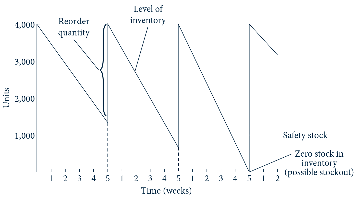
Figure 7: An organization selling 2,500 units before its next order will have to reorder 2,500 units plus the units it anticipates selling during the lead time. The amount ordered differs from one five-week period to the next (Coyle et al. 2020)

Figure 9.14 illustrates a fixed review every five weeks. The replenishment must replace the 2,500 units used before review and also cover expected demand during replenishment lead time so inventory can return to the 4,000-unit target. Because realized demand or lead time can vary, successive order quantities need not be equal.

“If demand and lead time are constant and known in advance, then an organization using the fixed order interval approach will periodically reorder exactly the same amount of inventory. If either demand or lead time varies, however, the amount ordered each time will vary, becoming a result of demand as well as lead time length.”

“For example, as Figure 9.14 indicates, an organization starting each period with 4,000 units and selling 2,500 units before its next order will have to reorder 2,500 units plus the units it anticipates selling during the lead time to bring inventory up to the desired beginning level of 4,000 units. Figure 9.14 shows an instance in which the amount ordered differs from one five-week period to the next.”

— Supply Chain Management: A Logistics Perspective (Coyle et al. 2020, 331, fig. 9.14).

Optimizing inventory ordering policies in practice

How to optimize the inventory policies of thousands of SKUs?

Automatically, with warehouse management systems (WMSs).

• Kanban system inventory ordering
  • Lean Manufacturing philosophy
  • Fixed lot sizes (order quantities)
  • Just-in-time (JIT) replenishment
    • Triggered at a certain inventory level
• Vendor-management inventory (VMI)

EOQ, JIT, and Kanban

“Establishing and implementing inventory policies can become complicated. Imagine what it might be like to optimize the inventory policies for 10,000 SKUs at the same time! For that reason, inventory policies usually are managed automatically by a warehouse management system or a material requirements planning system (see Chapter 11). One of the important innovations in the Lean Manufacturing philosophy (covered in detail in Chapter 16) is an approach to inventory ordering called kanban. In a kanban system, you pick a lot size for each SKU, and the lot size never changes. When you use all the items in a lot, another full lot is waiting behind it. When you start pulling from that second lot, the system automatically places an order for a new lot. A kanban system is an example of a replenishment policy that’s triggered at a certain inventory level and has a fixed order quantity (lot size). The kanban system is simple, and it prevents many expensive mistakes (such as overordering and stockouts) that can sometimes occur with more sophisticated inventory policies. Kanban systems help ensure that inventory arrives when it is needed, and not before, so it’s a form of just-in-time (JIT) replenishment.”

— Supply Chain Management For Dummies (Stanton 2023, 123).

References

Coyle, John Joseph, C. John Langley, Robert A. Novack, and Brian J. Gibson. 2020. Supply Chain Management: A Logistics Perspective. 11th edition. Cengage.

Erlenkotter, Donald. 1990. “Ford Whitman Harris and the Economic Order Quantity Model.” Operations Research 38 (6): 937–46.

Gitman, Lawrence J., Carl McDaniel, Amit Shah, et al. 2018. “Introduction to Business.” OpenStax, September 19. https://openstax.org/books/introduction-business/pages/10-4-pulling-it-together-resource-planning.

Harris, Ford Whitman. 1913. “How Many Parts to Make at Once.” Factory, The Magazine of Management.

King, Peter L. 2011. “Understanding Safety Stock and Mastering Its Equations.” APICS Magazine. https://web.mit.edu/2.810/www/files/readings/King_SafetyStock.pdf.

Lisan, Sharfuddin. 2018. “Safety Stock Determination of Uncertain Demand and Mutually Dependent Variables.” International Journal of Business and Social Research.

Richards, Gwynne. 2014. Warehouse Management: A Complete Guide to Improving Efficiency and Minimizing Costs in the Modern Warehouse. Second edition. Kogan Page Limited.

Stanton, Daniel. 2023. Supply Chain Management for Dummies. 3rd ed. John Wiley & Sons, Inc.

“Warehouse Vs. Inventory: Their Roles And Differences.” 2025. Inbound Logistics, February 3. https://www.inboundlogistics.com/articles/warehouse-vs-inventory/.