Layout and space allocation
A place for everything, and everything in its place Benjamin Franklin
🧠 Learning objectives
Differentiate the function of main warehouse areas and flows.
Formulate space allocation (SKU-to-flow) problems using mathematical optimization.
Discuss formulation assumptions, trade-offs, and caveats.
Functional areas
Receiving staging area
Cross-docking staging area
Bulk storage/reserve/unit-load area
Forward-, fast-, primary-picking area
Shipping area
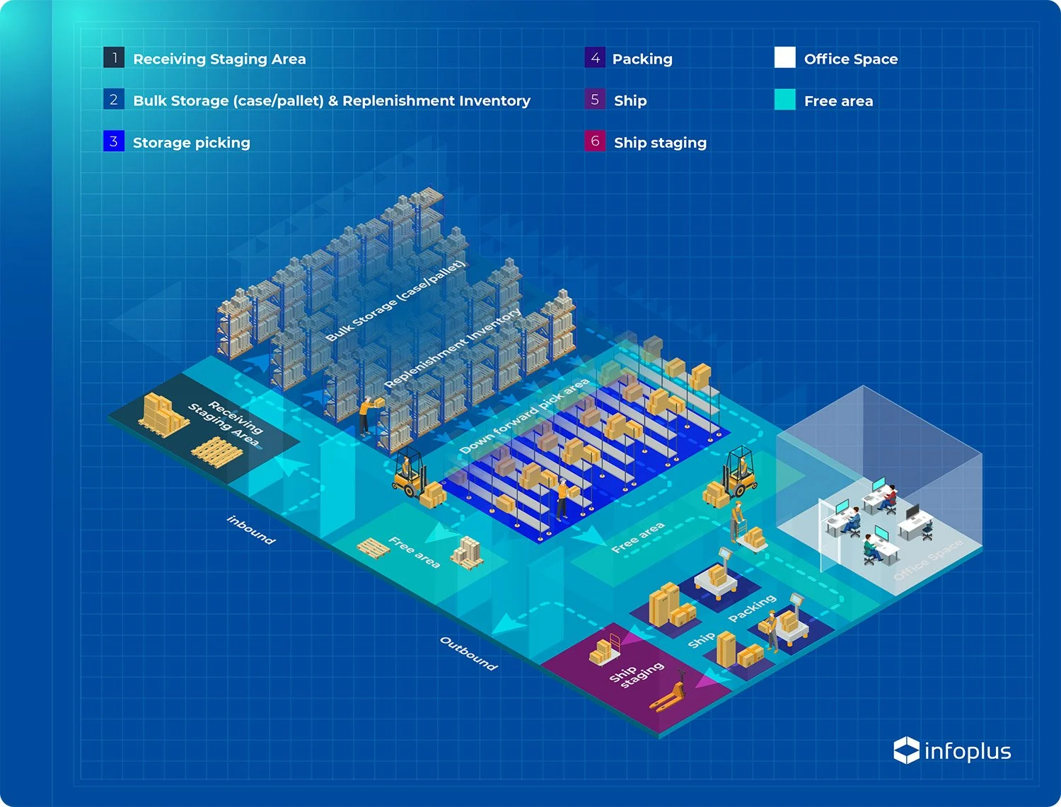
The five labels are functional areas in the cited warehouse model. Packing is treated as work that readies an order in the shipping area, not as a sixth independently modeled area. Staging is temporary: products then cross-dock to shipping or move into reserve or forward storage.
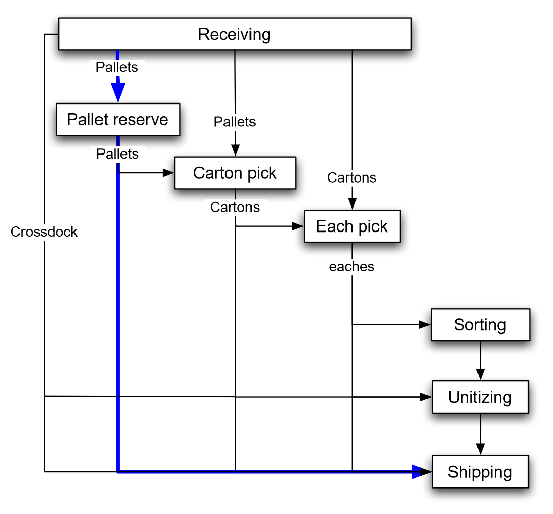
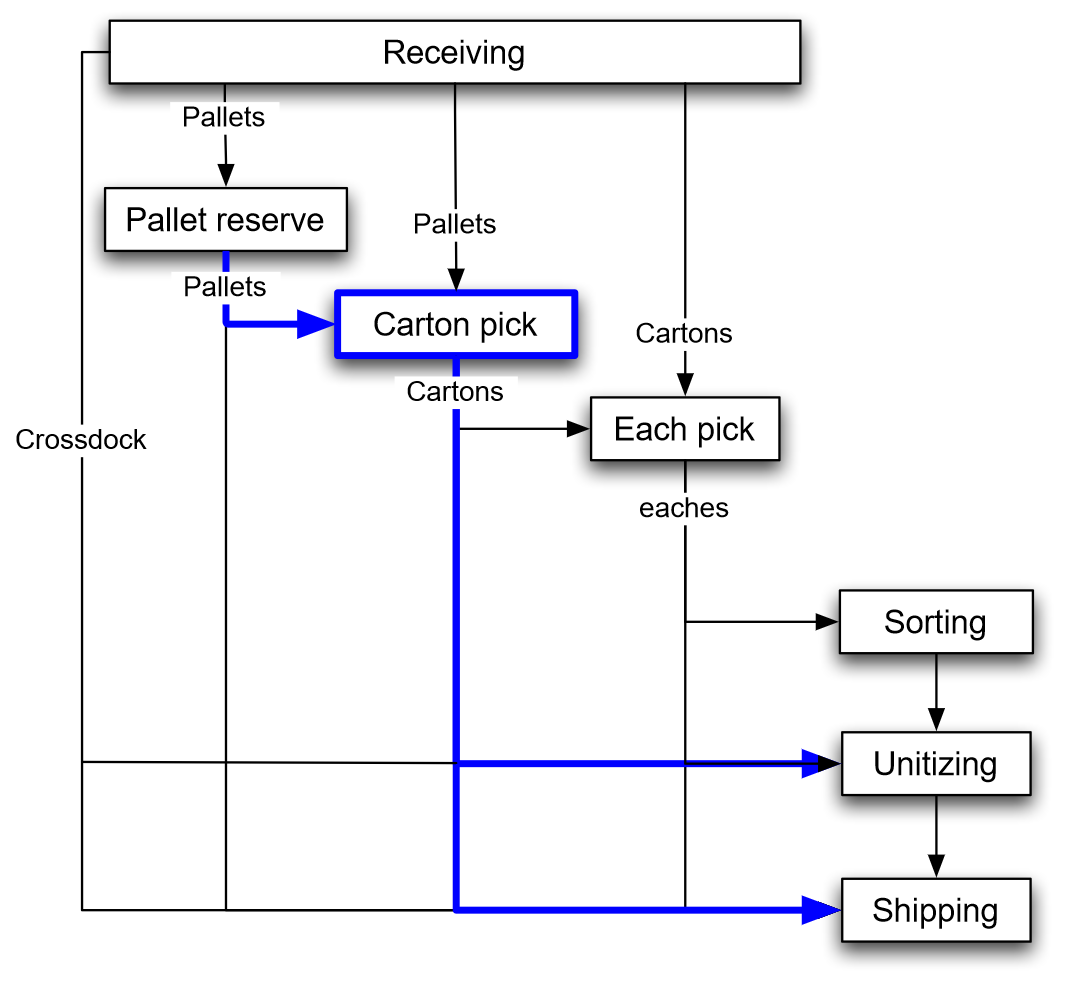
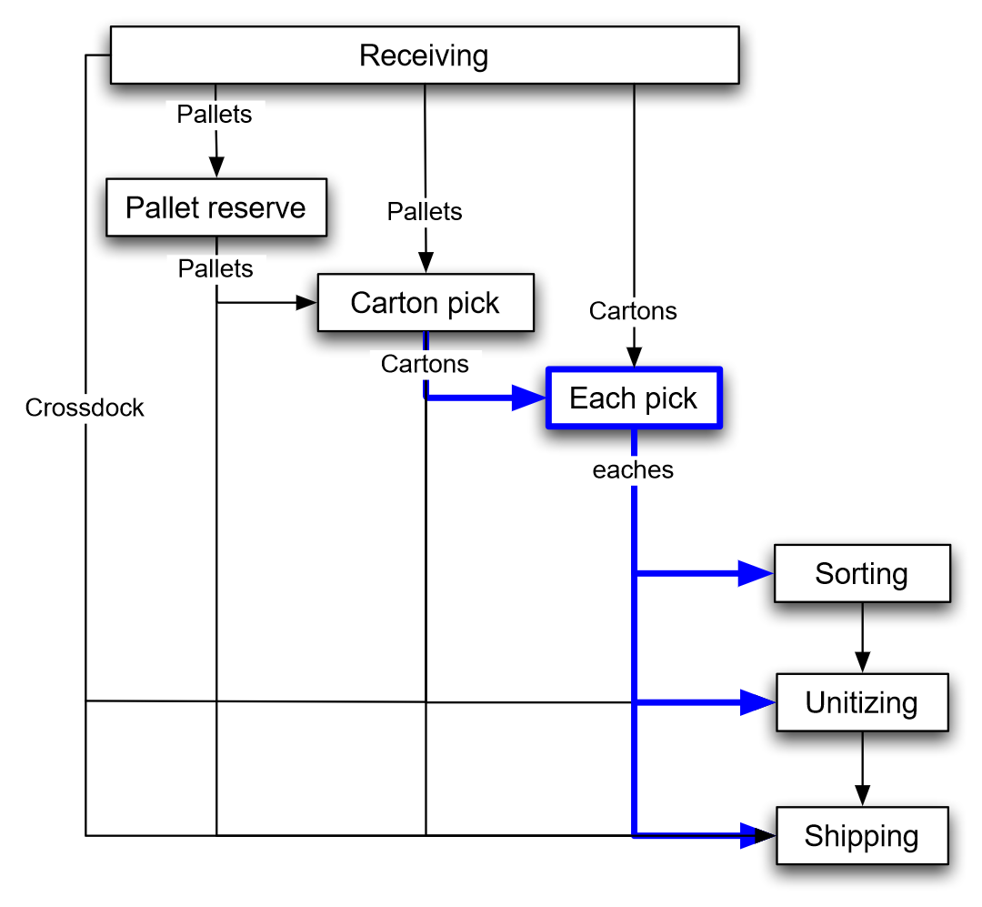
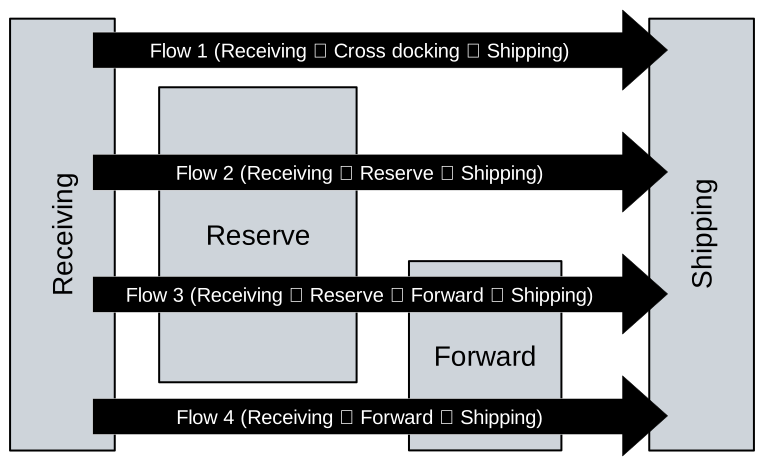
This paper considers warehouse configurations that include a subset of the following five functional areas: receiving, shipping, staging for cross-docking operation, reserve and forward. In the receiving area, pallet loads or individual cartons of products are received. If necessary, they are staged for a short period and then moved either to the shipping area directly (cross-docking operation) or to the storage area. In the shipping area, picked order items are readied (e.g. shrink-wrapped, packed) and staged (if necessary) for shipping to the next destination. In the staging area for cross-docking, products are sorted and accumulated for further outbound operations. The reserve area is a storage area for bulky product items that typically reside in the warehouse for a relatively longer duration. Normally, the reserve area uses high-density storage equipment to achieve the goal of high space utilization. The forward area is a relatively smaller storage area typically used for fast order picking or performing value-added operations or order collation. Thus, the following material flows are possible in a warehouse: Flow 1, receiving to cross-docking to shipping; Flow 2, receiving to reserve area to shipping; Flow 3, receiving to reserve area to forward area to shipping; and Flow 4, receiving to forward area to shipping.
Flow 1 is the cross-docking operation. Upon receipt, product items are either put into a staging area for a short period and then moved to the shipping area, or directly moved to the shipping area. The received products are typically presorted at suppliers’ facilities. The operation here is simply to pass on the product to a customer or the next facility in the supply chain.
Flow 3 is also a typical warehouse operation. Products are first stored in the reserve area typically in pallet loads, broken into smaller loads (cartons or cases) and then moved to the forward area for fast order picking, order consolidation or performing value added operations.
— Mathematical Model for Warehouse Design and Product Allocation (Heragu et al. 2005, 329–30 , sec. 3) .
Typical warehouse flows
The simplest type of warehouse is a unit-load warehouse, which means that only a single, common “unit” of material is handled at a time. The typical unit-load is a pallet. Because pallets are (mostly) standardized and are (mostly) handled one-at-a-time, both space and labor requirements scale: It takes about \(n\) times the space to store \(n\) pallets as for one; and it takes about \(n\) times the labor to handle \(n\) pallets as for one. An example of unit-load is a third-party transshipment warehouse that receives, stores, and forwards pallets. The third-party warehouse is a subcontractor to others for warehouse services. A third-party warehouse typically charges its customers for each pallet handled (received and later shipped); and rent for space occupied. In this chapter we study unit-load issues in the context of such a warehouse; but many warehouses have some portion of their activity devoted to moving unit-loads, as in Figure 6.1.
— Warehouse & Distribution Science (Bartholdi and Hackman 2019, 51 (PDF p. 74)) .
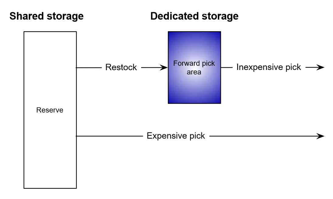
The handling unit carton or case is not standardized, but generally it refers to a rectangular box that weighs between about 5 and 50 pounds (2.3–22.7 kilograms); can be handled by one person; is conveyable (which depends on the type of conveyor); and can be stored on a pallet. When handled in volume, cartons are typically stored on pallets and so restocking is a unit-load process, but picking is not, which creates additional complexities in our models of space and labor. One consequence is that it becomes much more difficult to measure the convenience of an individual location; but it is still possible to make broad distinctions in convenience. A particularly convenient region that is replenished from within the warehouse is called a forward area or fast-pick area. The material flow on which we concentrate here is that of Figure 7.1.
— Warehouse & Distribution Science (Bartholdi and Hackman 2019, 77–78 (PDF p. 100)) .
Piece-picking is the most labor intensive activity in the warehouse because the product is handled at the smallest units-of-measure. Furthermore, the importance of piece-picking has greatly increased because of pressures to reduce inventory while expanding product lines. Warehouses that, 20 years ago, might have shipped cartons to customers now ship pieces and much more frequently. In a typical operation pieces are picked from cartons and neither picking nor restocking is unit-load, as shown in Figure 8.1. One of the first efficiencies a warehouse should consider is to separate the storage and the picking activities. A separate picking area, sometimes called a fast-pick or forward-pick or primary-pick area, is a sub-region of the warehouse in which one concentrates picks and orders within a small physical space. This can have many benefits, including reduced pick costs and increased responsiveness to customer demand. However, there is a science to configuring the fast-pick area.
— Warehouse & Distribution Science (Bartholdi and Hackman 2019, 99–100 (PDF p. 122)) .
Handling costs of different flows
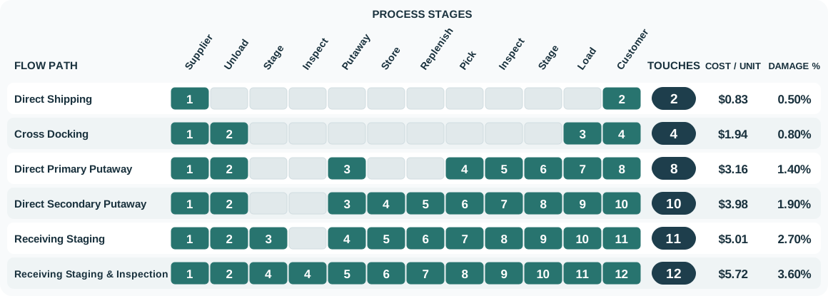
Figure 2 compares the touch sequence across six receiving flows. More touches typically coincide with higher unit costs and damage rates.
Figure 2: Six receiving flows. In this example, cost per unit means the handling cost of moving one case through the complete path; damage % is the share of cases damaged.
Receiving flow optimization (Frazelle 2016, 113 ) .
Direct Shipping
2
$0.83
0.50%
Cross Docking
4
$1.94
0.80%
Direct Primary Putaway
8
$3.16
1.40%
Direct Secondary Putaway
10
$3.98
1.90%
Receiving Staging
11
$5.01
2.70%
Receiving Staging & Inspection
12
$5.72
3.60%
Direct Shipping
A+ Cube Movers
A+ Reliability
Back Orders, Bulky Merchandise
Cross Docking
Consistent A Movers
A+ Reliability
Back Orders, Transfers, Customer Specials, Single SKU Unit Loads
Direct Primary Putaway
A, B & C Movers
A+ Reliability
Empty Primary
Direct Secondary Putaway
A, B & C Movers
A to B+ Reliability
Empty Secondary
Receiving Staging
A, B & C Movers
B Reliability
Quick Turn Trailers or Docks
Receiving Staging & Inspection
B & C Movers
B & C Reliability
Seasonal, High Variability
Direct shipping bypasses the warehouse completely, requiring two touches—one to load the outbound truck at the origin and one to receive the inbound truck at the destination.
Inbound loads are precisely and tightly scheduled into the warehouse, sorted immediately into outbound orders, and moved immediately to their outbound docks.
Direct primary put-away checks to see whether there are any empty primary locations and directs put-aways to those locations, thus bypassing receiving inspection, put-away, storage, and replenishment. Eight touches are required.
Direct secondary put-away bypasses receiving staging and inspection and moves product directly from unloading into reserve locations.
Traditional receiving requires staging at receiving, inspection, put-away to reserve storage, and replenishment to primary picking locations.
— World-Class Warehousing and Material Handling (Frazelle 2016, 111–12, 115 ) .
Bulk-storage/reserve/unit-load area
Only a single (“unit”) of material (e.g., pallet) handled at a time.
Many warehouses have part of their activity devoted to moving unit-loads.
How to increase space cost-efficiency (pallet-positions[^def_pallet_position]/unit area[^def_why_area])?
The simplest type of warehouse is a unit-load warehouse, which means that only a single, common “unit” of material is handled at a time. The typical unit-load is a pallet. Because pallets are (mostly) standardized and are (mostly) handled one-at-a-time, both space and labor requirements scale: It takes about \(n\) times the space to store \(n\) pallets as for one; and it takes about \(n\) times the labor to handle \(n\) pallets as for one. An example of unit-load is a third-party transshipment warehouse that receives, stores, and forwards pallets. The third-party warehouse is a subcontractor to others for warehouse services. A third-party warehouse typically charges its customers for each pallet handled (received and later shipped); and rent for space occupied. In this chapter we study unit-load issues in the context of such a warehouse; but many warehouses have some portion of their activity devoted to moving unit-loads, as in Figure 6.1.
One revenue source of the third-party warehouse is to charge rent by the pallet-month. But because the warehouse typically tallies its own expenses by the square-foot or square-meter (for example, rent of the building, climate control, cleaning, and so on), the warehouse naturally wants many pallet positions per unit area. It can achieve this in two ways: by taking advantage of vertical space and by using deep lanes.
— Warehouse & Distribution Science (Bartholdi and Hackman 2019, 51 ) .
Optimal lane depth
A lane is a row of pallet positions, one behind the other, accessed from a single aisle.
Shallow lanes
More space lost in aisles.
Increased accessibility.
Faster position reassignment.
Deep lanes
More space for pallet positions.
Reduced compliance with FIFO.
Increased S/R times.
Lane depth counts pallet positions behind one aisle access point. Deeper lanes spread aisle space across more positions, but they also delay reassignment of empty positions and can increase handling time. They do not automatically prevent FIFO: pallet-flow and drive-through rack can preserve FIFO under appropriate operating rules.
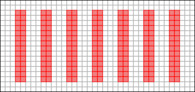
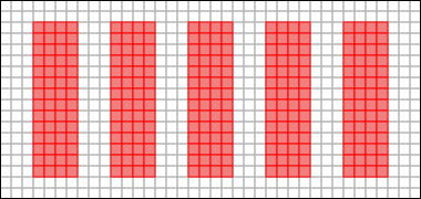
Aisles provide accessibility, not storage, and so this space for aisles is not directly revenue-generating. Consequently we prefer to reduce aisle space to the minimum necessary to provide adequate accessibility. For this the aisles must be at least wide enough for a forklift to insert or extract a pallet. By storing product in lanes, additional pallet positions can share the same aisle space and so amortize that cost. Should lanes be four pallets deep? Six? Ten? There are many issues to consider, but the most important one is effective utilization of space. For example, double-deep layout (lanes that are two pallet positions deep) fits about 41% more pallet positions in the same floor area than does single-deep layout in the example of Figure 6.3; but is it a better layout? Are enough of the additional pallet positions usefully engaged? There is a trade-off: The single-deep layout has eight aisles and provides 196 pallet storage locations, all of which are directly accessible, which means that they are available for reassignment as soon as the current pallet is shipped out. In contrast, the double-deep layout has only six aisles and provides 280 pallet storage locations—but only 140 of them are directly accessible. Moreover, the 140 that are directly accessible are not available for reuse until the interior pallet location in the same lane becomes available. So: Deeper lanes produce more pallet storage locations but they are of diminishing value.
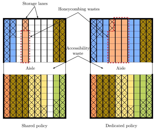
In most warehouses a lane is dedicated entirely to a single SKU to avoid double-handling pallets. This saves time but incurs a cost in space: When the first pallet is retrieved from a lane, that position is unoccupied but unavailable to other SKUs. The deeper the lane, the greater this cost. The first pallet position in a \(k\) -deep lane that holds uniformly moving product will be occupied only \(1/k\) of the time, the second \(2/k\) of the time, and so on (Figure 6.4). This waste is called honeycombing. Deeper lanes are more susceptible to honeycombing; but shallow lanes use more space for accessibility.
To maximize space efficiency SKU \(i\) should be stored in a lane of depth that minimizes floor space-time that is unoccupied but unavailable to other SKUs. The optimum lane depth can be determined by simply evaluating all possibilities, as has been done in Table 6.1. In Figure 6.5 waste has been plotted for each lane depth, and it can be seen that 2-deep lanes are most space efficient when the aisle is less than 4 pallet positions wide; otherwise 4-deep is best.
— Warehouse & Distribution Science (Bartholdi and Hackman 2019, 54–56 , secs. 6.1.2–6.1.3) .
Deep-lane storage reduces aisle space but loses use of pallet positions due to honey-combing, the creation of empty but unusable storage positions. (The positions cannot be used until the remaining product in the same column and/or aisle are removed.) The optimal lane depth balances these two losses to get the greatest (time-averaged) occupancy of floor space. Optimal lane depth are given by Theorems 6.2 and 6.3.
In laying out pallet storage there are other issues to consider besides space utilization. For example, in some warehouses, such as those of food distributors, it is important to move product in accordance with the rule of “First In First Out” (FIFO). Some special types of rack such as pallet flow rack support FIFO; but otherwise FIFO can be guaranteed only to within the lane depth. Making lanes deeper might give better space utilization; but it reduces compliance with FIFO. In addition, deeper lanes can increase insert/extract times.
— Warehouse & Distribution Science (Bartholdi and Hackman 2019, 69–70 , secs. 6.3–6.4) .
Lane depth and space utilization
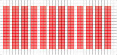
For example, pallet-position engagement (see Figure 3 ) varies by lane depth:
1-deep: 8 aisles and 196 directly accessible pallet positions.
2-deep: 6 aisles and 140 directly accessible pallet positions.
A pallet position consists of the pallet footprint plus any required clearance space.
Figure 3: The 2-deep layout fits 84 (42.86%) more pallet positions than the 1-deep layout. However, it may lead to increased handling times and reduced accessibility for certain SKUs.
Aisles provide accessibility, not storage, and so this space for aisles is not directly revenue-generating. Consequently we prefer to reduce aisle space to the minimum necessary to provide adequate accessibility. For this the aisles must be at least wide enough for a forklift to insert or extract a pallet.
By storing product in lanes, additional pallet positions can share the same aisle space and so amortize that cost. Should lanes be four pallets deep? Six? Ten? There are many issues to consider, but the most important one is effective utilization of space. For example, double-deep layout (lanes that are two pallet positions deep) fits about 41% more pallet positions in the same floor area than does single-deep layout in the example of Figure 6.3; but is it a better layout? Are enough of the additional pallet positions usefully engaged? There is a trade-off: The single-deep layout has eight aisles and provides 196 pallet storage locations, all of which are directly accessible, which means that they are available for reassignment as soon as the current pallet is shipped out. In contrast, the double-deep layout has only six aisles and provides 280 pallet storage locations—but only 140 of them are directly accessible. Moreover, the 140 that are directly accessible are not available for reuse until the interior pallet location in the same lane becomes available. So: Deeper lanes produce more pallet storage locations but they are of diminishing value.
By pallet position we mean the floor space required to hold a pallet. This includes not only the footprint of the pallet but also any required gap between one pallet and an adjacent one (Figure 6.4). Let the lanes be \(k\) pallet positions deep. Each lane requires aisle space at its head so that pallets can be inserted and removed. Let the aisle space in front of the pallet be of area \(a\) , measured in pallet positions. Then the total area charged to one lane is \(k + a/2\) pallet positions. This area is the sum of space devoted to storage (\(k\) ) and space that provides accessibility (\(a/2\) ).
In most warehouses a lane is dedicated entirely to a single SKU to avoid double-handling pallets. This saves time but incurs a cost in space: When the first pallet is retrieved from a lane, that position is unoccupied but unavailable to other SKUs. The deeper the lane, the greater this cost. The first pallet position in a \(k\) -deep lane that holds uniformly moving product will be occupied only \(1/k\) of the time, the second \(2/k\) of the time, and so on (Figure 6.4). This waste is called honeycombing. Deeper lanes are more susceptible to honeycombing; but shallow lanes use more space for accessibility.
Table 6.1 displays daily snapshots of a SKU with an order size that occupies four pallet positions and which is extracted at a rate of one pallet position per day. In single-deep rack, all the unused space is the aisle space required for accessibility. Deeper aisles require less aisle space per pallet position—but the additional pallet positions are less fully occupied.
To maximize space efficiency SKU \(i\) should be stored in a lane of depth that minimizes floor space-time that is unoccupied but unavailable to other SKUs. The optimum lane depth can be determined by simply evaluating all possibilities, as has been done in Table 6.1. In Figure 6.5 waste has been plotted for each lane depth, and it can be seen that 2-deep lanes are most space efficient when the aisle is less than 4 pallet positions wide; otherwise 4-deep is best.
— Warehouse & Distribution Science (Bartholdi and Hackman 2019, 54–56 ) .
Lane depth and storage policies
Dedicated policy:
Poor space utilization (“honeycombing”).
Efficient handling.
Randomized (shared) policy:
Efficient space utilization.
May incur pallet double handling (blockage issues).
Inventory/SKU is low -> Allow blockage.
Inventory/SKU is high -> No blockage.
The optimal lane depth minimizes floor space-time that is unoccupied but unavailable to other SKUs.
In laying out pallet storage there are other issues to consider besides space utilization. For example, in some warehouses, such as those of food distributors, it is important to move product in accordance with the rule of “First In First Out” (FIFO). Some special types of rack such as pallet flow rack support FIFO; but otherwise FIFO can be guaranteed only to within the lane depth. Making lanes deeper might give better space utilization; but it reduces compliance with FIFO. In addition, deeper lanes can increase insert/extract times.
Aisles provide accessibility, not storage, and so this space for aisles is not directly revenue-generating. Consequently we prefer to reduce aisle space to the minimum necessary to provide adequate accessibility. For this the aisles must be at least wide enough for a forklift to insert or extract a pallet. By storing product in lanes, additional pallet positions can share the same aisle space and so amortize that cost. Should lanes be four pallets deep? Six? Ten? There are many issues to consider, but the most important one is effective utilization of space. For example, double-deep layout (lanes that are two pallet positions deep) fits about 41% more pallet positions in the same floor area than does single-deep layout in the example of Figure 6.3; but is it a better layout? Are enough of the additional pallet positions usefully engaged? There is a trade-off: The single-deep layout has eight aisles and provides 196 pallet storage locations, all of which are directly accessible, which means that they are available for reassignment as soon as the current pallet is shipped out. In contrast, the double-deep layout has only six aisles and provides 280 pallet storage locations—but only 140 of them are directly accessible. Moreover, the 140 that are directly accessible are not available for reuse until the interior pallet location in the same lane becomes available. So: Deeper lanes produce more pallet storage locations but they are of diminishing value.
In most warehouses a lane is dedicated entirely to a single SKU to avoid double-handling pallets. This saves time but incurs a cost in space: When the first pallet is retrieved from a lane, that position is unoccupied but unavailable to other SKUs. The deeper the lane, the greater this cost. The first pallet position in a \(k\) -deep lane that holds uniformly moving product will be occupied only \(1/k\) of the time, the second \(2/k\) of the time, and so on (Figure 6.4). This waste is called honeycombing. Deeper lanes are more susceptible to honeycombing; but shallow lanes use more space for accessibility.
To maximize space efficiency SKU \(i\) should be stored in a lane of depth that minimizes floor space-time that is unoccupied but unavailable to other SKUs. The optimum lane depth can be determined by simply evaluating all possibilities, as has been done in Table 6.1. In Figure 6.5 waste has been plotted for each lane depth, and it can be seen that 2-deep lanes are most space efficient when the aisle is less than 4 pallet positions wide; otherwise 4-deep is best.
— Warehouse & Distribution Science (Bartholdi and Hackman 2019, 54–56, 69–70 ) .
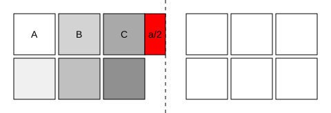
Exercise 1 Space utilization in a warehouse laneConsider the pallet positions A, B, C, shown in Figure 5 . If the warehouse has a single SKU occupying these positions and the demand is 1 pallet per day. Each pallet position occupies area \(p\) and the aisle space in front of the pallet is of area \(a/2\) .
What is the utilization rate \(u_{A}\) , \(u_{B}\) , and \(u_{C}\) for each position?
What is the total unoccupied area across the three days for the lane in terms of \(p\) and \(a\) ?
Figure 5: Pallet positions A, B, and C with area \(p\) and aisle front area \(a/2\) . SKU demand is 1 pallet per day.
Exercise 1 Space utilization in a warehouse lane
We analyze the occupancy of each pallet position over three days, given that one pallet is removed each day from the front position (i.e., position C). The utilization rate for each position is:
\(u_{A} = 1\) \(u_{B} = 2/3\) \(u_{C} = 1/3\)
The total unoccupied area-days for the lane is calculated as follows:
Day 1: \(\frac{a}{2}\)
Day 2: \(p + \frac{a}{2}\)
Day 3: \(2p + \frac{a}{2}\)
Total: \(3p + \frac{3a}{2}\)
Lane depth and storage equipment
The choice of storage equipment should align with the warehouse’s operational goals, SKU characteristics, and handling requirements.
Lane depth and aisle width
Aisle space is not directly revenue-generating, so minimizing aisle width is desirable.
The aisle must be wide enough to accommodate the material handling equipment (MHE) used in the warehouse.
Narrowing the aisle to 1 gives 336 pallet positions: 140 (71.43%) more than the 1-deep layout in Figure 3 (a) , and 56 (20.00%) more than the 2-deep layout in Figure 3 (b) . Both comparison layouts use aisle width 3.
Figure 6: Warehouse layout with narrow aisles. More space is available for storage.
The capacity percentages on this slide are generated by the displayed course layout, so they are model outputs rather than values reported by the source. The general mechanism is that aisle width must satisfy equipment access requirements; changing the rack or truck can reduce access space, but it also changes equipment, floor, guidance, and operating requirements.
Aisles provide accessibility, not storage, and so this space for aisles is not directly revenue-generating. Consequently we prefer to reduce aisle space to the minimum necessary to provide adequate accessibility. For this the aisles must be at least wide enough for a forklift to insert or extract a pallet. By storing product in lanes, additional pallet positions can share the same aisle space and so amortize that cost. Should lanes be four pallets deep? Six? Ten? There are many issues to consider, but the most important one is effective utilization of space. For example, double-deep layout (lanes that are two pallet positions deep) fits about 41% more pallet positions in the same floor area than does single-deep layout in the example of Figure 6.3; but is it a better layout? Are enough of the additional pallet positions usefully engaged? There is a trade-off: The single-deep layout has eight aisles and provides 196 pallet storage locations, all of which are directly accessible, which means that they are available for reassignment as soon as the current pallet is shipped out. In contrast, the double-deep layout has only six aisles and provides 280 pallet storage locations—but only 140 of them are directly accessible. Moreover, the 140 that are directly accessible are not available for reuse until the interior pallet location in the same lane becomes available. So: Deeper lanes produce more pallet storage locations but they are of diminishing value.
— Warehouse & Distribution Science (Bartholdi and Hackman 2019, 54–55 , sec. 6.1.2) .
Selective rack or single-deep rack stores pallets one deep, as in Figure 5.1. Due to rack supports each pallet is independently accessible, and so any SKU can be retrieved from any pallet location at any level of the rack. This gives complete freedom to retrieve any individual pallet but requires relatively more aisle space to access the pallets.
Double-deep rack essentially consists of two single-deep racks placed one behind the other, and so pallets are stored two deep. Due to rack supports each 2-deep lane is independently accessible, and so any SKU can be stored in any lane at any level of the rack. To avoid double-handling, it is usual that each lane be filled with a single SKU, which means that some pallet locations will be unoccupied whenever some SKU is present in an odd number of pallets. Another disadvantage of deep lanes is that slightly more work is required to store and retrieve product. However, deep lanes have the advantage of requiring fewer aisles to access the pallets, which means that the warehouse can hold more product. A special truck is required to reach past the first pallet position.
Reach and double-reach lift truck is equipped with a reach mechanism that allows its forks to extend to store and retrieve a pallet. The double-reach truck is required to access the rear positions in double deep rack storage. Each truck requires an aisle width of 7–9 feet (2.1–2.7 meters), their lift height is limited to 30 feet (9.1 meters), and they travel at about 50 feet/minute (15.2 meters/minute).
— Warehouse & Distribution Science (Bartholdi and Hackman 2019, 39–41 , sec. 5.1.1) .
Lane depth and MHE
Aisle size and space savings involve a compromise between MHE requirements and costs and the savings achieved by narrower aisles.
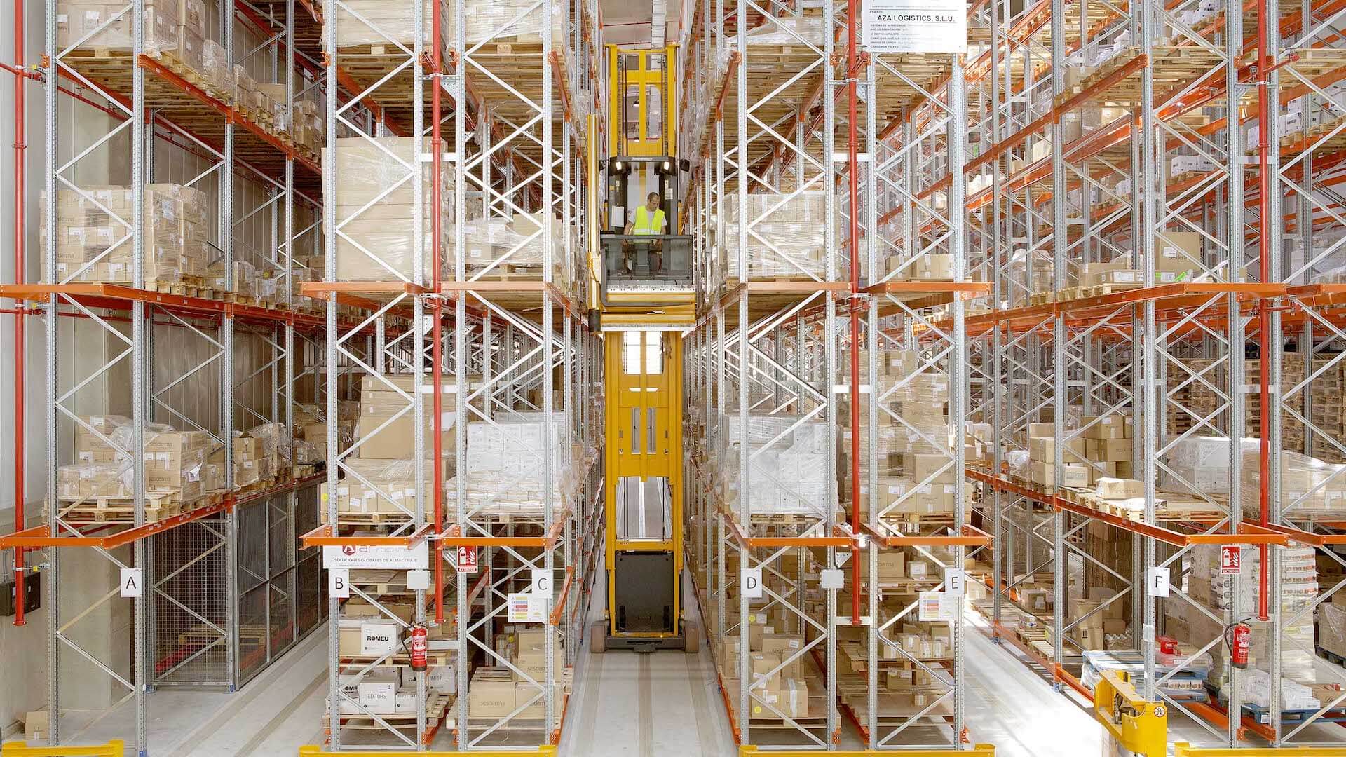
Example: Very Narrow Aisle (VNA) forklifts can operate in aisles as narrow as 1.5 m (see, e.g., Figure 7 ).
Figure 7: Example of VNA forklift (ArRacking Storage Solutions ).
Double-deep rack essentially consists of two single-deep racks placed one behind the other, and so pallets are stored two deep. Another disadvantage of deep lanes is that slightly more work is required to store and retrieve product. However, deep lanes have the advantage of requiring fewer aisles to access the pallets, which means that the warehouse can hold more product. A special truck is required to reach past the first pallet position. Drive-in or drive-through rack allows a lift truck to drive within the rack frame to access the interior loads.
Except for automated storage-and-retrieval systems (AS/RS), some type of lift truck is required to access the loads in pallet rack; and specialized racks may require specialized trucks. A double-reach lift truck is required to access the rear positions in double-deep rack storage.
— Warehouse & Distribution Science (printed pp. 39–41; PDF pp. 61–63) (Bartholdi and Hackman 2019, 39–41 ) .
Optimal lane depth for block stacking
Block stacking involves storing pallets of a single Stock Keeping Unit (SKU) in floor lanes, stacked to a fixed height, and accessed from one side.
Two primary sources of space inefficiency arise in this system:
Honeycombing waste within lanes.
Accessibility waste for aisles that provide access.
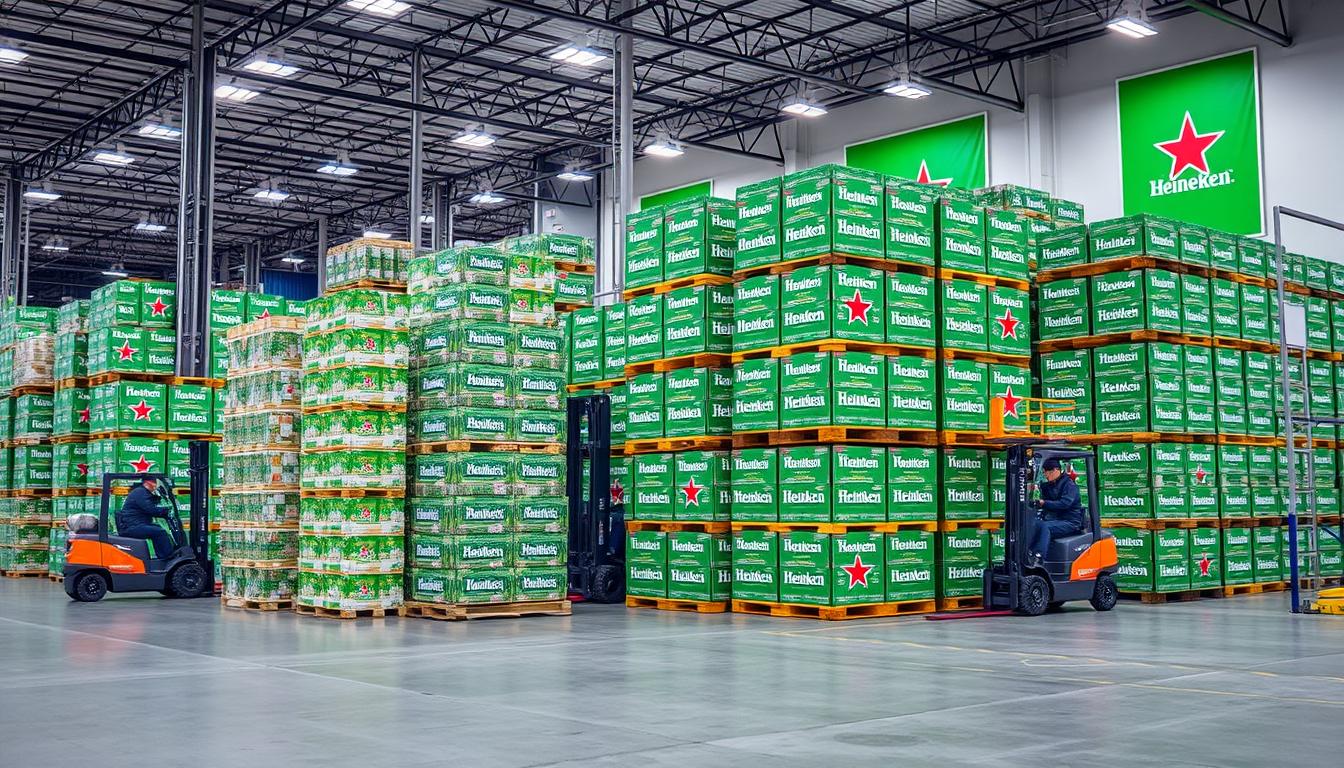
Figure 8: Block stacking is a common practice in beverage and food warehouses, optimizing space utilization while maintaining accessibility.
Block stacking is a floor-storage system rather than a rack system. A lane is normally dedicated to one SKU to avoid relocations, so empty positions behind or beneath accessible stock can become temporarily unusable. The cited model supports broad manufacturing and distribution-center use; the photograph is an example and does not establish how prevalent the method is in beverage or food warehouses.
Block stacking is an inexpensive and conventional storage system whose performance depends on the efficient use of space. It is a unit load storage system in which pallets of stock keeping units (SKUs) are stacked on top of one another in lanes on the warehouse floor. Pallets are stacked to the maximum stacking height which depends on the conditions and heights of the pallets, load weights, safety limits, clearance height of the warehouse and so on. No racking or storage facility is required for this system and it can be employed in any warehouse with wide floor space. This makes it an inexpensive storage system to implement but challenging to manage in terms of space planning.
When the inventories of the SKUs are big enough to justify assigning a lane to a single SKU, no blockage policy is enforced. In this case, to avoid blockage and relocation, a lane is dedicated to a SKU once it occupies the first position of the lane. This case mainly occurs in the warehouses located in manufacturing systems or the distribution centres where plenty of pallets of different SKUs are block-stacked. However, this restriction wastes storage spaces in a lane when it is filled or depleted as there will be some unoccupied pallet positions in the lane that are just available to the pallets of the assigned SKU. This effect is termed honeycombing and waste associated with it is incurred to the system until a lane becomes entirely occupied or empty. In addition to honeycombing, aisles also contribute to the overall wasted space. Aisles are required to have access to the lanes but their devoted spaces are not directly used for storage.
— Optimising Space Utilisation in Block Stacking Warehouses (Derhami et al. 2017, 6436–37 , sec. 1) .
Storing a batch of pallets in deep lanes increases the honeycombing waste, but the space required for aisles decreases, while the reverse is true for the shallow lanes. Hence, a trade-off between the lane depth and width must be considered to optimise space utilisation.
Minimising the waste of storage space maximises space utilisation. So, one can obtain the optimal lane depth that maximises the space utilisation by deriving a mathematical expression to calculate waste of storage space and then finding the optimal lane depth that minimises this waste expression. The waste of storage space is obtained by calculating three types of waste: (1) waste of storage space caused by honeycombing, \(W_H\) ; (2) waste of storage space dedicated to the aisles, \(W_A\) ; and (3) waste of unoccupied storage space on top of the occupied lanes, \(W_U\) .
— Optimising Space Utilisation in Block Stacking Warehouses (Derhami et al. 2017, 6437–39 , secs. 1 and 3) .
Optimal lane depth: Problem description
Consider a block stacking warehouse where:
SKUs are stored in lanes of fixed depth.
Lanes are last-in first-out (LIFO) (i.e., the most recently added pallet is the first to be removed).
Lanes are accessible from one side (i.e., the front).
Batch arrivals are deterministic (i.e., known arrival times and quantities).
Batch arrivals are either:
instantaneous (i.e., all pallets arrive at once), or
at finite rate (i.e., pallets arrive over time).
Goal: Determine the optimal common lane depth that minimizes average space waste across all SKUs, where average space waste is defined as the sum of honeycombing and aisle accessibility waste.
Let \(N\) be the number of SKUs. For each SKU \(i \in \{1,\dots,N\}\) :
\(Q_i\) : batch size in pallets.\(P_i\) : production or storage rate in pallets per hour.\(\lambda_i\) : depletion or demand rate in pallets per hour.\(Z_i\) : stack height in pallets.\(A\) : aisle width in pallet units.\(Z_i*x_c\) : total lane depth in pallet units, where \(x_c\) is the common lane depth to be determined. Objective. Find the optimal common lane depth \(x_c^*\) that minimizes average space waste across all SKUs.
Most convenient locations: flow-through layout
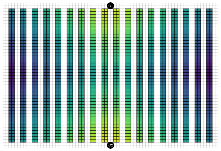
What are the most convenient storage locations of unit-load U-shaped and I-shaped warehouses?
Figure 9: Flow-through layout. Lighter cells mark storage locations closer to the input/output (I/O) positions.
In a flow-through layout, receiving and shipping lie on opposite sides, so product generally crosses the building. The source explains the resulting convenience pattern and why the best geometry depends on SKU velocity. The Manhattan-distance shading and the exact I/O coordinates in the figure are course-model choices.
The layout of the warehouse determines the cost associated with each storage location. In the layout of Figure 6.10 the average positions of receiving and shipping are in the middle of opposite sides of the warehouse. This is sometimes referred to as a flow-through configuration because all product flows from one side of the facility to the other. As a result all the storage locations along one side of an aisle are equally convenient.
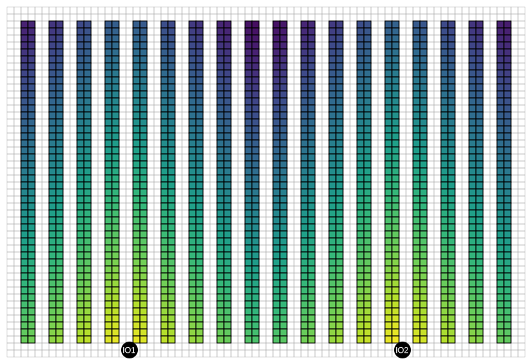
If both receiving and shipping are on the same side of the warehouse this induces a different economic terrain within, as shown in Figure 6.11. Because product flows in and out the same side of the warehouse, this is sometimes referred to as a U-flow configuration.
Now the best storage locations, which are at the middle of the common receiving and shipping dock, are very convenient indeed because a location that is close to receiving would also be close to shipping. However, there are relatively few such prime locations and there are more inconvenient locations than before; and the least convenient locations, at the far top corners are even less convenient than the least convenient of Figure 6.10.
Which layout is better? In this case, as with so many of the design decisions, it depends on the populations of SKUs passing through the warehouse. If there are few very fast-moving SKUs, as is typical in cosmetics, apparel, or other fashion businesses, it may be more efficient to put receiving and shipping on the same side of the facility, because the savings from the few very convenient locations may offset any loss due to the greater number of less convenient locations.
— Warehouse & Distribution Science (Bartholdi and Hackman 2019, 65–67 , sec. 6.2.3) .
Most convenient locations: U-shaped layout
Figure 10: U-shaped layout. Lighter cells mark storage locations closer to the input/output (I/O) positions and shorter travel distance.
Now the best storage locations, which are at the middle of the common receiving and shipping dock, are very convenient indeed because a location that is close to receiving would also be close to shipping. However, there are relatively few such prime locations and there are more inconvenient locations than before; and the least convenient locations, at the far top corners are even less convenient than the least convenient of Figure 6.10.
Which layout is better? In this case, as with so many of the design decisions, it depends on the populations of SKUs passing through the warehouse. If there are few very fast-moving SKUs, as is typical in cosmetics, apparel, or other fashion businesses, it may be more efficient to put receiving and shipping on the same side of the facility, because the savings from the few very convenient locations may offset any loss due to the greater number of less convenient locations.
U-flow configuration: Receiving and shipping are located on the same side of the warehouse. This makes the most convenient locations still more convenient and less convenient locations even worse. It is appropriate when product movement has strong ABC skew (that is, when very few SKUs account for most of the activity). It provides dock flexibility for both shipping and receiving: If one experiences a surge of activity, it can make use of additional doors from the other function. It permits more efficient use of forklifts: When a forklift reports for an assignment, it may be given a put-away and a retrieval, matched to reduce dead-heading. It minimizes truck apron and roadway and allows expansion along the other three sides of the warehouse.
— Warehouse & Distribution Science (Bartholdi and Hackman 2019, 65–67 ) .
Fast-, forward-, or primary-pick area
Sub-region of the warehouse (warehouse-within-warehouse):
Most popular SKUs in small amounts.
Picks concentrated in small space.
Reduced pick costs and increased responsiveness .
Less unproductive travel time (prime real estate).
Piece-picking is the most labor intensive activity in the warehouse because the product is handled at the smallest units-of-measure. Furthermore, the importance of piece-picking has greatly increased because of pressures to reduce inventory while expanding product lines. Warehouses that, 20 years ago, might have shipped cartons to customers now ship pieces and much more frequently. In a typical operation pieces are picked from cartons and neither picking nor restocking is unit-load, as shown in Figure 8.1. One of the first efficiencies a warehouse should consider is to separate the storage and the picking activities. A separate picking area, sometimes called a fast-pick or forward-pick or primary-pick area, is a sub-region of the warehouse in which one concentrates picks and orders within a small physical space. This can have many benefits, including reduced pick costs and increased responsiveness to customer demand. However, there is a science to configuring the fast-pick area.
— Warehouse & Distribution Science (Bartholdi and Hackman 2019, 99 ) .
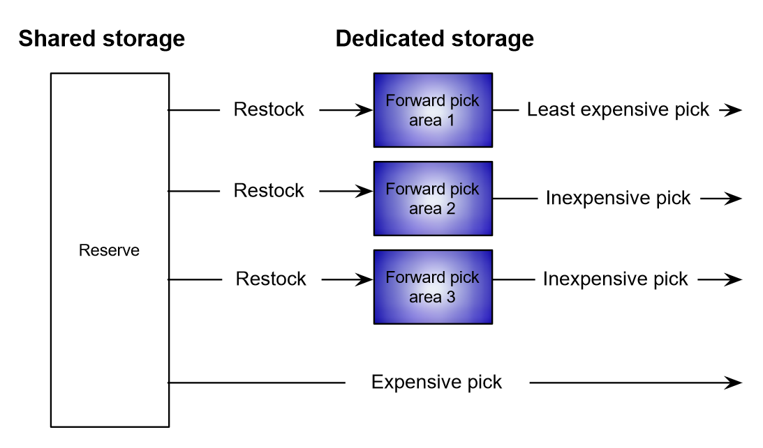
Multiple fast-pick areas
Figure 12: Pick areas may have different economics (e.g., flow-rack or carousel) (Bartholdi and Hackman 2019 ) .
Suppose there are \(m\) fast-pick areas, each with its own economics: savings per pick (compared to from reserve) and restock costs, as suggested by Figure 8.6. Now the question becomes which SKUs go to which fast-pick areas and which to reserve. Each of the \(n\) SKUs can be picked from at most one area. Brute-force search can find the best stocking strategy within \(O(m^n)\) steps by enumerating all possible assignments of SKUs to storage modes and then evaluating the result. However, this is completely impractical for realistic values (\(m = 2, 3\) and \(n\) on the order of tens of thousands).
Some optimal stocking strategy has the following structure: If all SKUs are ranked by bang-for-buck then the top \(k_1\) SKUs would be assigned to the storage mode with largest savings per pick, the next \(k_2\) would be assigned to the next best storage mode, and so on. Note that “best storage” depends only on savings per pick and is independent of restock costs.
— Warehouse & Distribution Science (Bartholdi and Hackman 2019, 120–21 ) .
Setting up a forward-pick area
Main questions when setting up a fast-picking area:
Which SKUs to store?How much of each SKU to store?
Trade-off: The fast-pick area may require replenishment from reserve .
The fast-pick area of a warehouse functions as a “warehouse within the warehouse”: Many of the most popular stock keeping units (SKUs) are stored there in relatively small amounts, so that most picking can be accomplished within a relatively small area. This means that pickers do less unproductive travel and may be more easily supervised. The trade-off is that the fast-pick area may require replenishment from bulk storage, or reserve. The basic issues in the design of a fast-pick area are: Which SKUs to store in the fast-pick area? And how much of each SKU to store?
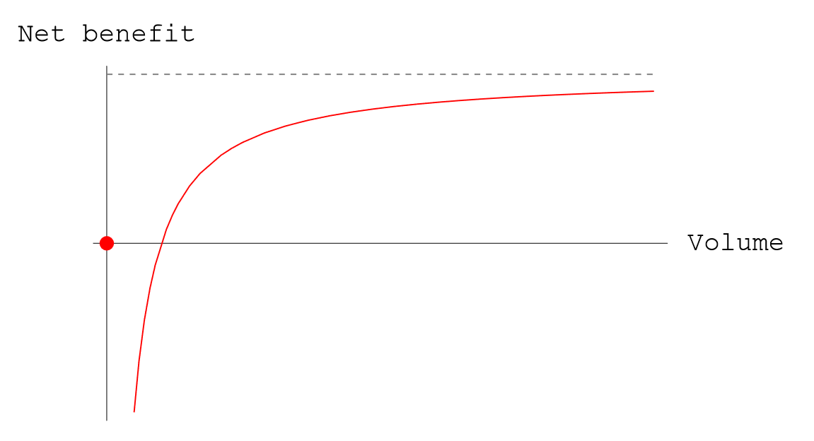
The net benefit realized by storing a SKU as a function of the quantity stored. The net benefit is zero if SKU \(i\) is not stored in the forward area; but if too little is stored, restock costs consume any pick savings. Note that from the shape of the objective function there is a minimum sensible amount of each SKU to store in the fast-pick area.
— Warehouse & Distribution Science (Bartholdi and Hackman 2019, 99, 113 ) .
Design model for warehouse space allocation
Figure 14: Typical warehouse product flow (based on Heragu 2022 ) .
The design problem joins two decisions: select one material flow for each product and size the functional areas required by those assignments. Its objective trades annual handling cost against area-dependent storage cost. Inventory price and carrying rate help estimate EOQ and dwell time; inventory holding cost is not an additional term in the model objective.
The two primary functions of a warehouse include (1) temporary storage and protection of goods and (2) providing value added services such as fulfilment of individual customer orders, packaging of goods, after sales services, repairs, testing, inspection and assembly. To perform the above functions, the warehouse is divided into several functional areas such as reserve storage area, forward (order collation) area and cross-docking. The paper presents a mathematical model and a heuristic algorithm that jointly determine product allocation to the functional areas in the warehouse as well as the size of each area using data readily available to a warehouse manager.
— Mathematical Model for Warehouse Design and Product Allocation (Heragu et al. 2005, 327 , abstract) .
The next section presents a mathematical model that determines the flow to which each product must be assigned and as result, the size of the functional areas within the warehouse. It assumes the following: available total storage space is known; expected time a product spends on the shelves is known (the dwell time); cost of handling each product in each flow is known; dwell time and cost have a linear relationship; annual product demand rates are known; and storage policies and material-handling equipment are known and these affect the unit handling and storage costs.
— Mathematical Model for Warehouse Design and Product Allocation (Heragu et al. 2005, 330–31 , secs. 3–4) .
The dwell time is the average duration a product stays on the shelf and is assumed to be known or can be estimated by the warehouse manager. In fact, based on annual product demand \(\lambda_i\) , order cost \(A_i\) , price per unit load of product \(P_i\) and carrying cost rate \(r\) , a simple economic order quantity (EOQ) model can be used to determine the optimal order quantity \(Q_i\) , as well as the average time a unit load of product spends on the shelves. For example, since the time between two successive replenishments is \(Q_i/\lambda_i\) , the average dwell time per unit load of product \(i\) is \(T_i=Q_i/(2\lambda_i)\) . Note that \(Q_i/2=\lambda_iT_i\) and this value or another reasonable estimate must be used in the objective function, which minimizes the total cost of handling the average, annual loads of each product assigned to its respective area as well as the corresponding annual storage costs.
The reader should not confuse storage costs with inventory holding costs. While inventory holding costs depend only upon the value of the inventory, they are the same whether the inventory is in reserve or forward or cross-docking area. Storing costs, on the other hand, depend upon the area in which the product is stored and these costs tend to carry a premium for the cross-docking and forward areas (because these are considered prime real estate in a warehouse) and are relatively not that expensive for the reserve area. Of course, the handling costs are different (in fact, the opposite) for these areas and thus our model trades off storage costs against handling costs.
— Mathematical Model for Warehouse Design and Product Allocation (Heragu et al. 2005, 332–33 , sec. 4) .
Exercise 2 Role of functional areas in a warehouseIn Table 1 , match each row in the “Functions” column with the appropriate Functional Area : 1) Receiving, 2) Shipping, 3) Staging for Cross-Docking, 4) Reserve, and 5) Forward.
Subset of functional areas: storage
Reserve area
Typically bulky product items
Relatively extended periods
Shipped as is (or with minimal “value-added” operations)
High-density storage equipment
Focus on high space utilization
Forward area
Smaller storage area
Fast order picking
Value-added operations
Order collation
In this section, we consider warehouse configurations that include a subset of the following five functional areas: receiving, shipping, staging for cross-docking operation, reserve, and forward.
In the receiving area, pallet loads or individual cartons of products are received. If necessary, they are staged for a short period and then either moved to the shipping area directly (cross-docking operation) or to the storage area. In the shipping area, picked order items are readied (e.g., shrink-wrapped, packed) and staged (if necessary) for shipping to the next destination.
In the staging area for cross-docking, products are sorted and accumulated for further outbound operations.
Reserve area is a storage area for bulky product items that typically reside in the warehouse for a relatively longer duration. Normally, the reserve area uses high-density storage equipment to achieve the goal of high space utilization.
Forward area is a relatively smaller storage area typically used for fast order picking or performing value-added operations or order collation. Thus, the following material flows are possible in a warehouse: Flow 1: receiving to cross-docking to shipping; Flow 2: receiving to reserve area to shipping; Flow 3: receiving to reserve area to forward area to shipping; and Flow 4: receiving to forward area to shipping.
— Mathematical Model for Warehouse Design and Product Allocation (Heragu et al. 2005, 329–30 ) .
Indexes (products, flows)
Parameters (costs, prices, EOQ, dwell time)
The slide writes annual demand as \(D_i\) ; Heragu et al. use \(\lambda_i\) for the same role. \(C_i^{\mathrm{order}}\) is currency per replenishment, \(P_i\) is currency per unit load, and \(C^{\mathrm{carry}}\) is a fraction per year. Their product, \(P_iC^{\mathrm{carry}}\) , is therefore a holding cost in currency per unit load per year. \(Q_i\) is the replenishment quantity, and \(T_i=Q_i/(2D_i)\) is average dwell time under the EOQ inventory-cycle assumptions.
The next section presents a mathematical model that determines the flow to which each product must be assigned and as result, the size of the functional areas within the warehouse. It assumes the following: available total storage space is known; expected time a product spends on the shelves is known (the dwell time); cost of handling each product in each flow is known; dwell time and cost have a linear relationship; annual product demand rates are known; and storage policies and material-handling equipment are known and these affect the unit handling and storage costs.
— Mathematical Model for Warehouse Design and Product Allocation (Heragu et al. 2005, 330–31 , secs. 3–4) .
The dwell time is the average duration a product stays on the shelf and is assumed to be known or can be estimated by the warehouse manager. In fact, based on annual product demand \(\lambda_i\) , order cost \(A_i\) , price per unit load of product \(P_i\) and carrying cost rate \(r\) , a simple economic order quantity (EOQ) model can be used to determine the optimal order quantity \(Q_i\) , as well as the average time a unit load of product spends on the shelves. For example, since the time between two successive replenishments is \(Q_i/\lambda_i\) , the average dwell time per unit load of product \(i\) is \(T_i=Q_i/(2\lambda_i)\) . Note that \(Q_i/2=\lambda_iT_i\) and this value or another reasonable estimate must be used in the objective function, which minimizes the total cost of handling the average, annual loads of each product assigned to its respective area as well as the corresponding annual storage costs.
— Mathematical Model for Warehouse Design and Product Allocation (Heragu et al. 2005, 332–33 , sec. 4) .
It is worth pausing to point out some implications of this model that will be useful in the context of warehouses. First, the average inventory over time is \(Q/2\) . This means that the average time in inventory of this particular item is \(Q/(2D)\) . This expression is frequently called turnover time. The inverse value is the average number of inventory turns. Note that the number of turns is not the same—indeed, is twice the value of—the number of times the item is ordered and replenished.
The obvious question to ask is what is the best quantity \(Q\) to order? To answer this we must enlarge the model by including some costs. The main costs common to inventories are the costs of reordering and the costs of holding inventory.
An order cycle is initiated by the placing of the order, which incurs cost \(c_T\) . Thereafter, holding costs are accrued for inventory-time (for example, widget-years), which is the area under the inventory curve. Summing these two cost components gives the total cost of one inventory cycle: \(c_T+c_H Q^2/(2D)\) . The cost per unit time is given by dividing the cost per cycle by the duration \(Q/D\) of a cycle, which gives \(c_TD/Q+c_HQ/2\) . Minimizing this rate of cost gives the economic order quantity: \(Q^*=\sqrt{2Dc_T/c_H}\) .
— Warehouse & Distribution Science (Bartholdi and Hackman 2019, 295–96 , appendix A.1) .
For a given product \(i\) :
\(C_{i}^{\mathrm{order}}\) : order cost\(D_{i}\) : annual demand rate\(C_{i}^{\mathrm{carry}}\) : inventory carrying cost rate/unit/year\(P_i\) : price per unit load\(P_iC_{i}^{\mathrm{carry}}\) : inventory carrying cost/unit/year
The optimal order quantity is \[
Q_i = \sqrt{\frac{2D_{i}C_{i}^{\mathrm{order}}}{P_iC^{\mathrm{carry}}}}
\]
Example of EOQ calculation:
\(C_{i}^{\mathrm{order}}\) = $200 per order\(D_{i}\) = 3,600 units/year\(C_{i}^{\mathrm{carry}}\) = 25%\(P_i\) = $100 per unit\(P_iC_{i}^{\mathrm{carry}} = 100 \times 25\% = \$25\) /unit/year
The optimal order quantity is:
\[
\begin{align}
Q_i = & \sqrt{\frac{2 \times 3,600 \times 200}{25}} \\
= & 240 \; \text{units}\\
\end{align}
\]
Parameters (product to flow handling & storage)
Product flows and the break-bulk factor
Model product flows.
Flow 3 is the only modeled flow that changes unit-load size: reserve storage handles supplier pallet loads, while the forward area handles the resulting cartons or cases. For example, \(d_i=\frac{\text{pallet-load size}}{\text{carton-load size}}\geq1\) . The ratio \(d_i\) describes the size conversion. The factor \(q_{i3}=\lceil d_i\rceil+1\) is a handling-count multiplier, not only a physical pallet-to-carton conversion factor, and the flow-3 handling and storage costs must be aggregated accordingly.
Flow 3 is also a typical warehouse operation. Products are first stored in the reserve area typically in pallet loads, broken into smaller loads (cartons or cases) and then moved to the forward area for fast order picking, order consolidation or performing value added operations.
— Mathematical Model for Warehouse Design and Product Allocation (Heragu et al. 2005, 329–30 , sec. 3) .
The exception is for products assigned to flow 3 because these products have different unit load sizes in the two areas encompassing flow 3. The unit load size of products assigned to flow 3 could be equal to that received from the suppliers in the reserve area, but different when handled in the forward area. This occurs because a pallet load is broken down to cases or cartons in the forward area. This is only for products assigned to flow 3. Hence, we introduce \(d_i\) to denote the ratio of the size of the unit load in the reserve area to that in the forward area and \(q_{ij}\) for \(j=3\) accounts for the fact that product \(i\) is handled \(\lceil d_i\rceil+1\) times. \(H_{ij}\) and \(C_{ij}\) should therefore correspond to aggregate handling and storage costs for \(j=3\) .
— Mathematical Model for Warehouse Design and Product Allocation (Heragu et al. 2005, 332–33 , sec. 4) .
Storage vs. inventory holding costs
Inventory holding costs (\(C^{\mathrm{carry}}\) ) depend only on the value of the inventory.
Same whether the inventory is in reserve or forward or cross-docking area.
Storage costs (\(C_{ij}^{\mathrm{store}}\) ) depend on the area in which the product is stored.
Costs tend to carry a premium for the cross-docking and forward areas (prime real estate in a warehouse).
Costs tend to be cheaper for the reserve area .
The reader should not confuse storage costs with inventory holding costs. While inventory holding costs depend only on the value of the inventory, they are the same whether the inventory is in reserve or forward or cross-docking area. Storing costs, on the other hand, depend on the area in which the product is stored, and these costs tend to carry a premium for the cross-docking and forward areas (because these are considered prime real estate in a warehouse) and are relatively not that expensive for the reserve area.
— Facilities Design (Heragu 2022, 289 ) .
Storage and handling costs
Storage costs (\(C_{ij}^{\mathrm{store}}\) ) of product \(i\) in material flow \(j\) are a function of:
The size of a product’s unit load.
Warehouse leasing/construction costs per square meter.
Shelving type used in each area encompassing flow \(j\) . Handling costs (\(C_{ij}^{\mathrm{handle}}\) ) of product \(i\) in material flow \(j\) are a function of:
Product size .
Product handling characteristics .
Material handling system used in the area(s) included in flow \(j\) .
We believe much of the input data such as the type and number of products, annual demand for each, order cost, unit price, and carrying cost rate are readily available to the warehouse designer. The storage cost \(C_{ij}\) is typically a function of the size of a product’s unit load, warehouse leasing or construction costs per square foot, as well as the type of shelving used in each area encompassing flow \(j\) . \(C_{ij}\) and \(H_{ij}\) for flow 3 must be aggregated to account for the fact that a pallet load could be broken down into cases or cartons. The cost of handling a unit load of product \(i\) in each flow \(j\) is a function of the product size, its handling characteristics, and the MHS used in the area(s) included in flow \(j\) . Chapter 3 provides a simple formula to estimate these costs based on labor, nonlabor, and prorated capital recovery costs of the MHS. Adapting this formula to the warehouse application is left as an exercise (see Exercise 29). The model (8.2) through (8.11) can be solved optimally using available mixed-integer programming software, and even large-scale problems with 75,000 items can be solved.
— Facilities Design (Heragu 2022, 290 ) .
Parameters (space allocation)
The source notation uses \(TS\) for total available storage space, \(S_i\) for the space required by one unit load, \(a\) , \(b\) , and \(c\) for the available vertical levels in cross-dock, reserve, and forward areas, and lower/upper limits for each area. The slide renames these quantities to make the area explicit. \(S^{\mathrm{total}}\) is storage space, not total building area; multiplying it by a consistent vertical-level factor gives the capacity used in the area constraints.
The next section presents a mathematical model that determines the flow to which each product must be assigned and as result, the size of the functional areas within the warehouse. It assumes the following: available total storage space is known; expected time a product spends on the shelves is known (the dwell time); cost of handling each product in each flow is known; dwell time and cost have a linear relationship; annual product demand rates are known; and storage policies and material-handling equipment are known and these affect the unit handling and storage costs.
— Mathematical Model for Warehouse Design and Product Allocation (Heragu et al. 2005, 330–31 , secs. 3–4 and notation block) .
Constraints (3)–(5) ensure that the space constraints for the cross-docking, reserve and forward areas are met. The right-hand side includes three additional variables whose sum is required to be 1 (constraint 6). This is to ensure 100% of the space available is allocated to the three areas. Constraints (7)–(9) serve to enforce upper and lower limits on the space that can be allocated to cross-docking, forward and reserve areas.
— Mathematical Model for Warehouse Design and Product Allocation (Heragu et al. 2005, 331–33 , model 1 and explanatory text) .
Variables
The source uses binary \(X_{ij}\) to select exactly one flow \(j\) for product \(i\) . The slide’s \(x_{ij}\) is the same assignment decision. The continuous variables \(w^{\mathrm{CD}}\) , \(w^{\mathrm{R}}\) , and \(w^{\mathrm{F}}\) are nonnegative proportions of available storage space assigned to cross-dock, reserve, and forward areas. In this model their sum is one, which also implies that each is at most one. If the equality were relaxed to permit unused storage space, explicit upper bounds or an unassigned-space variable would be needed.
The next section presents a mathematical model that determines the flow to which each product must be assigned and as result, the size of the functional areas within the warehouse. It assumes the following: available total storage space is known; expected time a product spends on the shelves is known (the dwell time); cost of handling each product in each flow is known; dwell time and cost have a linear relationship; annual product demand rates are known; and storage policies and material-handling equipment are known and these affect the unit handling and storage costs.
— Mathematical Model for Warehouse Design and Product Allocation (Heragu et al. 2005, 330–31 , secs. 3–4 and notation block) .
Constraints (3)–(5) ensure that the space constraints for the cross-docking, reserve and forward areas are met. The right-hand side includes three additional variables whose sum is required to be 1 (constraint 6). This is to ensure 100% of the space available is allocated to the three areas. Constraints (7)–(9) serve to enforce upper and lower limits on the space that can be allocated to cross-docking, forward and reserve areas.
— Mathematical Model for Warehouse Design and Product Allocation (Heragu et al. 2005, 331–33 , model 1 and explanatory text) .
Objective function
Minimize total material handling and storage costs:
\[
\min \sum_{i=1}^{n}{\sum_{j=1}^{4}{(2C_{ij}^{\mathrm{handle}})D_{i}q_{ij}x_{ij}}} + \sum_{i=1}^{n}{\sum_{j=1}^{4}{\frac{Q_{i}}{2}C_{ij}^{\mathrm{store}}q_{ij}x_{ij}}}
\]
Handling costs
\(2C_{ij}^{\mathrm{handle}}\) = the model assumes two handling transactions per product \(i\) (receiving, shipping); adjust this factor for flows with more touches.\((2C_{ij}^{\mathrm{handle}})D_{i}\) = annual handling costs
Storage costs
\(\frac{Q_{i}}{2}\) = avg. annual load of \(i\) \(\frac{Q_{i}}{2}C_{ij}^{\mathrm{store}}\) = avg. yearly storage cost of product \(i\) in material flow \(j\)
The model also assumes that each product incurs two material-handling transactions—one for receiving and another for shipping, regardless of the area it is assigned to. If products assigned to a particular flow require more than two (or only one) material-handling transactions, the coefficient of the corresponding terms in the objective function must be appropriately weighted. For example, in some cases, the products assigned to the combined forward/reserve flow may incur three transactions, one for receiving at the reserve area, another for shipping to the forward area, and a third for shipping. If this is the case, that term must have a coefficient of 3.
— Facilities Design (Heragu 2022, 289 ) .
Constraints: SKU-to-flow
Each SKU is assigned to only one type of material flow :
\[
\begin{align}
\sum_{j}^{4}{x_{ij}} = 1 & \quad \text{for} \; i = 1,2,3, \dots, n \\
\end{align}
\]
If a single product could be allocated to multiple flows :
Create additional product versions with demands proportional to the different flow ratios.
Notice that, despite the initial estimate, the model may provide a different assignment based on the total costs.
Example: A manager estimates that a product has demand of 10,000 units and is likely to be split in a 7:3 ratio between reserve and cross-docking. This ratio results in creating two artificial products with demands of 7,000 and 3,000 units.
Constraint (2) ensures that each product is assigned to only one type of material flow. If the same product could be allocated to multiple flows due to different demand patterns, then our model requires that the manager at least knows or can estimate the percentage of this product that could be assigned to two or more of the four flows. For modeling purposes, additional versions of this product are then created (depending upon how many flows this product could be assigned to) with the demand data appropriately reduced. For example, assume that 70% of a certain product whose demand is 10,000 units per year on average is likely to be assigned to one of the four flows, say reserve storage, and another 30% to another, say cross-docking. For modeling purposes, an additional version of this product is therefore created with demand equal to 7,000 and 3,000 for the two products. Note that although the manager might assume that the product is likely to be split on a 7:3 ratio to reserve:cross-docking, the model may provide a different assignment based on the total costs.
— Mathematical Model for Warehouse Design and Product Allocation (Heragu et al. 2005, 333 ) .
Constraints: Functional area space
The SKUs assigned to each area are such that their collective space requirement is within the allotted cubic space .
\[
\begin{align}
\sum_{i=1}^{n}{\frac{Q_{i}}{2}S_{i}x_{i1}} &\leq w^{\mathrm{CD}} (z^{\mathrm{CD}}S^{\mathrm{total}}) & \text{Cross docking (flow 1)} \\
\sum_{i=1}^{n}{\frac{Q_{i}}{2}S_{i}x_{i2}} + \sum_{i=1}^{n}{\frac{Q_{i}}{2}\rho_{i}^{\mathrm{R}}S_{i}x_{i3}} &\leq w^{\mathrm{R}}(z^{\mathrm{R}} S^{\mathrm{total}}) & \text{Reserve (flows 2 and 3)}\\
\sum_{i=1}^{n}{\frac{Q_{i}}{2}(1-\rho_{i}^{\mathrm{R}})S_{i}x_{i3}} + \sum_{i=1}^{n}{\frac{Q_{i}}{2}S_{i}x_{i4}} &\leq w^{\mathrm{F}} (z^{\mathrm{F}}S^{\mathrm{total}}) & \text{Forward (flows 3 and 4)}\\
\end{align}
\]
Notice that \(\rho_{i}^{\mathrm{R}}\) is the average percentage of time a unit load of product \(i\) spends in the reserve area when assigned to flow \(3\) .
Each inequality compares required average storage capacity with the capacity allotted to one functional area. The factor \(Q_i/2\) is average inventory under the EOQ cycle. Assignment \(x_{ij}\) activates the relevant flow contribution. Flow 3 is split: \(\rho_i^{\mathrm{R}}\) allocates its average load to reserve, and \(1-\rho_i^{\mathrm{R}}\) allocates the remainder to forward. The right-hand side multiplies the area’s space share by its vertical levels and total available storage space.
The dwell time is the average duration a product stays on the shelf and is assumed to be known or can be estimated by the warehouse manager. In fact, based on annual product demand \(\lambda_i\) , order cost \(A_i\) , price per unit load of product \(P_i\) and carrying cost rate \(r\) , a simple economic order quantity (EOQ) model can be used to determine the optimal order quantity \(Q_i\) , as well as the average time a unit load of product spends on the shelves. For example, since the time between two successive replenishments is \(Q_i/\lambda_i\) , the average dwell time per unit load of product \(i\) is \(T_i=Q_i/(2\lambda_i)\) . Note that \(Q_i/2=\lambda_iT_i\) and this value or another reasonable estimate must be used in the objective function, which minimizes the total cost of handling the average, annual loads of each product assigned to its respective area as well as the corresponding annual storage costs.
— Mathematical Model for Warehouse Design and Product Allocation (Heragu et al. 2005, 332–33 , sec. 4) .
Constraints (3)–(5) ensure that the space constraints for the cross-docking, reserve and forward areas are met. The right-hand side includes three additional variables whose sum is required to be 1 (constraint 6). This is to ensure 100% of the space available is allocated to the three areas. Constraints (7)–(9) serve to enforce upper and lower limits on the space that can be allocated to cross-docking, forward and reserve areas.
— Mathematical Model for Warehouse Design and Product Allocation (Heragu et al. 2005, 331–33 , model 1, constraints 3–5) .
Constraints: All available space is allocated
Ensures 100% of the space available is allocated to the three areas:
\[
\begin{align}
w^{\mathrm{CD}} + w^{\mathrm{R}} + w^{\mathrm{F}} = 1 \quad
\end{align}
\]
This equality is a deliberate modeling assumption: all available storage space is divided among cross-dock, reserve, and forward areas. It does not mean that every square meter of the building—including docks, aisles, offices, or support space—is assigned by these variables. If unused storage capacity is permitted, replace the equality with an inequality or add an explicit unassigned-space variable so the accounting remains complete.
Constraints (3)–(5) ensure that the space constraints for the cross-docking, reserve and forward areas are met. The right-hand side includes three additional variables whose sum is required to be 1 (constraint 6). This is to ensure 100% of the space available is allocated to the three areas. Constraints (7)–(9) serve to enforce upper and lower limits on the space that can be allocated to cross-docking, forward and reserve areas.
— Mathematical Model for Warehouse Design and Product Allocation (Heragu et al. 2005, 331–33 , model 1, constraint 6 and explanatory text) .
Constraints: Space lower and upper limits
Enforce upper and lower limits on the space that can be allocated to the cross-docking, forward, and reserve areas:
\[
\begin{align}
LL_{\mathrm{CD}}\leq w^{\mathrm{CD}} (z^{\mathrm{CD}}S^{\mathrm{total}}) \leq UL_{\mathrm{CD}}\quad \\
LL_{\mathrm{R}} \leq w^{\mathrm{R}} (z^{\mathrm{R}} S^{\mathrm{total}}) \leq UL_{\mathrm{R}}\quad \\
LL_{\mathrm{F}} \leq w^{\mathrm{F}} (z^{\mathrm{F}} S^{\mathrm{total}}) \leq UL_{\mathrm{F}}\quad
\end{align}
\]
The slide rewrites Heragu’s symbols in course notation. Here, \(LL_{\mathrm{CD}},LL_{\mathrm{R}},LL_{\mathrm{F}}\) and \(UL_{\mathrm{CD}},UL_{\mathrm{R}},UL_{\mathrm{F}}\) are lower and upper area bounds; \(w^{\mathrm{CD}},w^{\mathrm{R}},w^{\mathrm{F}}\) are vertical storage levels; \(z^{\mathrm{CD}},z^{\mathrm{R}},z^{\mathrm{F}}\) are allocated proportions; and \(S^{\mathrm{total}}\) is total available floor area. Their product therefore has area units and must remain between the corresponding bounds.
Parameters
\(a,b,c\) : Levels of space available in the vertical dimension in each functional area, \(a\) , cross-docking; \(b\) , reserve; and \(c\) , forward\(S_i\) : Space required for storing a unit load of product \(i\) \(TS\) : Total available storage space\(Q_i\) : Order quantity for product (in unit loads)\(T_i\) : Dwell time (in years) per unit load of product \(i\) \(LL_{\mathrm{CD}}, UL_{\mathrm{CD}}\) : Lower and upper storage space limit for the cross-docking area\(LL_{\mathrm{F}}, UL_{\mathrm{F}}\) : Lower and upper storage space limit for the forward area\(LL_{\mathrm{R}}, UL_{\mathrm{R}}\) : Lower and upper storage space limit for the reserve area.
Decision variables
\(X_{ij}=1\) if product \(i\) is assigned to flow type \(j\) ; 0 otherwise\(\alpha,\beta,\gamma\) : Proportion of available space assigned to each functional area; \(\alpha\) , cross-docking; \(\beta\) , reserve; \(\gamma\) , forward.
— Facilities Design (Heragu 2022, sec. 8.6.5 , “Design Model for Warehouse Space Allocation,” printed pp. 287–288) .
Constraint (8.3) ensures that each product is assigned to only one type of material flow. If the same product could be allocated to multiple flows due to different demand patterns, then our model requires that the manager to estimate the percentage of this product that could be assigned to two or more of the four flows. For modeling purposes, additional versions of this product are then created (depending on how many flows this product could be assigned to) with the demand data appropriately reduced. For example, let us assume that 70% of a certain product whose demand is 10,000 units per year on average is likely to be assigned to the reserve storage area, and another 30% to cross-docking. For modeling purposes, an additional version of this product is therefore created with demand equal to 7000 and 3000 for the two products. Note that although the manager may assume that the product is likely to be split on a 7:3 ratio to reserve/cross-docking, the model may provide a different assignment based on the total costs. Constraints (8.4) through (8.6) ensure that the space constraints for the cross-docking, reserve, and forward areas are met. The right-hand side includes three additional variables whose sum is required to be 1 (constraint 8.7). This is to ensure that 100% of the space available is allocated to the three areas. Constraints (8.8) through (8.10) serve to enforce upper and lower limits on the space that can be allocated to the cross-docking, forward, and reserve areas.
— Facilities Design (Heragu 2022, sec. 8.6.5 , “Design Model for Warehouse Space Allocation,” printed pp. 289–290) .
The printed equation (8.9) repeats the cross-docking bound; the middle row on this slide uses the reserve symbols identified by the parameter list and the following explanation.
Exercise 3 Adjusting the model: One product, multiple flowsConsider that product \(p\) has demand of 10,000 units and is likely to be split in a 7:3 ratio between reserve and cross-docking. However, the variable \(x_{ij}\) , where \(i\) is the product and \(j\) is the flow, is binary and can only be assigned to a single flow:
\[
\sum_{j}^{4} x_{ij} = 1 \quad \forall \quad i = 1, 2, 3, \ldots, n
\]
How can we adjust the model to deal with this specific situation?
Replace product \(p\) with two artificial product versions:
\(p_1\) : demand of 7,000 units.\(p_2\) : demand of 3,000 units.
Each version can be assigned to one flow. The model then chooses the assignments that minimize total cost.
The adjustment preserves the model’s exactly-one-flow binary assignment. It represents one physical SKU by two artificial product records, with annual demands of 7,000 and 3,000 units. The product index set and parameter rows expand, but the variable domain does not change. A formulation that lets one product variable take fractional shares across flows would be a different model extension.
Constraint (2) ensures that each product is assigned to only one type of material flow. If the same product could be allocated to multiple flows due to different demand patterns, then our model requires that the manager at least knows or can estimate the percentage of this product that could be assigned to two or more of the four flows. For modeling purposes, additional versions of this product are then created (depending upon how many flows this product could be assigned to) with the demand data appropriately reduced. For example, assume that 70% of a certain product whose demand is 10,000 units per year on average is likely to be assigned to one of the four flows, say reserve storage, and another 30% to another, say cross-docking. For modeling purposes, an additional version of this product is therefore created with demand equal to 7,000 and 3,000 for the two products. Note that although the manager might assume that the product is likely to be split on a 7:3 ratio to reserve:cross-docking, the model may provide a different assignment based on the total costs.
— Mathematical Model for Warehouse Design and Product Allocation (Heragu et al. 2005, 333 , sec. 4) .
Summary
Model simultaneously considers the product allocation and functional area sizing problems in the design of a warehouse.
Solve the two problems jointly to minimize annual handling and storage costs .
Required input data are readily available in most warehouses.
The model can be solved to optimality for 3,000 SKUs using commercial MILP solvers.
For larger problems (e.g., 150,000 SKUs), see (meta-)heuristic solutions in (Heragu et al. 2005 ) .
For a multi-step approach that includes decisions on functional areas, travel distances, and storage strategies (e.g., dedicated, class-based, randomized), see Huuskes (2023 ) .
This paper has simultaneously considered the product allocation and functional area size determination problems in the design of a warehouse. It provides a mathematical model and a heuristic algorithm to solve the two problems jointly so that annual handling and storage costs can be minimized. The input data requirement for this model is readily available in most warehouses and the model considers realistic constraints. We believe this is the only available model that considers the two problems simultaneously and allows the user to solve them optimally.
— Mathematical Model for Warehouse Design and Product Allocation (Heragu et al. 2005, 337 ) .