| To | 0 | A | B | C | D |
|---|---|---|---|---|---|
| From | |||||
| 0 | 0 | 12 | 7 | 11 | 10 |
| A | 12 | 0 | 10 | 5 | 6 |
| B | 7 | 10 | 0 | 11 | 15 |
| C | 11 | 5 | 11 | 0 | 13 |
| D | 10 | 6 | 15 | 13 | 0 |
9 Uncertainty and Disturbances in Logistics
Metaheuristics and Disturbances
Keywords
metaheuristics, simulated annealing, tabu search, genetic algorithms, randomness, diversification, intensification, local optima, disturbances
“One does not discover new lands without consenting to lose sight of the shore for a very long time.” — André Gide
While local search methods are effective at improving solutions, they often get trapped in local optima—valleys in the solution landscape from which no small move can escape. Metaheuristics provide a higher-level framework to guide these subordinate heuristics, orchestrating the search process to find better global solutions.
This module explores how metaheuristics balance intensification (refining good solutions) and diversification (exploring new areas through smartly designed perturbations).
Finally, we discuss strategies for handling dynamic disturbances in logistics. So far, you have been working with static problems, where all information is available at the start. In practice, many logistics problems are dynamic, in which new information arrives over time, and possibly stochastic, meaning that some information is uncertain but follow known probability distributions (e.g., expected demand). We will discuss how to adapt your algorithms to handle these challenges.
After this module, you should be able to:
- Distinguish between local search and metaheuristics.
- Explain the roles of intensification and diversification in search algorithms.
- Implement trajectory-based metaheuristics like Simulated Annealing and Tabu Search.
- Understand how randomness helps escape local optima.
- Discuss strategies for handling dynamic disturbances in logistics.
9.1 Exercises
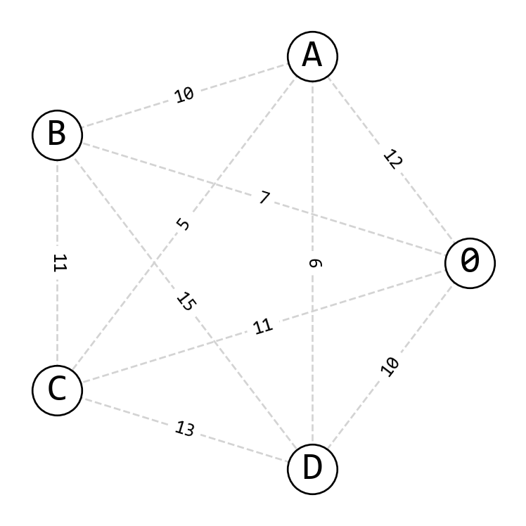
Exercise 9.1 Tabu Search. Use Tabu Search to optimize the route for a traveling salesman problem. This problem involves 4 customers who need to be visited sequentially before returning to the starting point, labeled 0. Refer to Figure 9.1 for the network representation.
Task: Design the following variations of the Tabu Search algorithm considering different strategies to store tabus in a short-term memory of the search. Provide the pseudocode for each variation and discuss its advantages and disadvantages.
Stores Entire Solutions Indefinitely: Once a solution is visited, it is added to the Tabu list and is never allowed to be revisited. For example, if the solution
(0, A, B, C, D, 0)is explored, it is added to the Tabu list, and the algorithm is prohibited from revisiting this exact sequence again at any point in the future.Stores Only the Moves with a Tenure of 2 Iterations: Instead of storing the entire solution, specific moves (like swapping two nodes or reversing a subsection of the tour) are tabu. For example, if the move was swapping customer B with customer D resulting in the route
(0, A, D, C, B, 0), then this specific swap is forbidden for the next two iterations.Stores the Moves and Their Corresponding Objective Function Values with a Tenure of 2 Iterations: This strategy involves recording the moves along with the objective function values (such as the total distance of the route) and prohibiting these specific move-cost combinations for two iterations. For instance, if swapping B and D resulted in a route cost of 350, the move (swap B and D) and this cost value are tabu. If the algorithm encounters the same move leading to the same or a worse cost within the tenure period, it is rejected.
Consider these settings:
- Travel Distance: Use the symmetric distance matrix presented in Table 9.1.
- Objective Function: Minimize the total travel distance.
- Search Space: All unique permutations of the customer nodes divided by 2 (a route and its reversed are equivalent), totaling \(\frac{4!}{2}\) = 12 tours (see Table 9.2).
- Termination Criterion: Stop after 3 iterations without any improvement.
- Tabu Tenure: Number of iterations a move is considered tabu so the search can explore different portions of the search space.
- Aspiration Criterion: Accept a tabu move if it yields a solution superior to the best current one.
- Initial Solution: \(S_0\) = (0→A→B→C→D→0).
- Neighborhood Structure: In local or tabu search, each iteration explores a set of neighboring solutions \(N(S)\)—a subset of the search space—formed by applying a single local transformation to the current solution \(S\). Examples:
- Swap-Based Neighborhood Structure. A swap move involves interchanging the positions of two customers (see example in Table 9.3).
- Reinsertion-Based Neighborhood Structure. A reinsertion move entails removing a customer from their current position in the route and inserting them into another position (see example in Table 9.4).
| # | Tour | Cost |
|---|---|---|
| 1 | (0→A→D→C→B→0) | 49 |
| 2 | (0→A→D→B→C→0) | 55 |
| 3 | (0→A→B→C→D→0) | 56 |
| 4 | (0→B→D→A→C→0) | 44 |
| 5 | (0→B→C→A→D→0) | 39 |
| 6 | (0→C→B→A→D→0) | 48 |
| 7 | (0→B→A→C→D→0) | 45 |
| 8 | (0→C→A→B→D→0) | 51 |
| 9 | (0→B→A→D→C→0) | 47 |
| 10 | (0→A→B→D→C→0) | 61 |
| 11 | (0→A→C→B→D→0) | 53 |
| 12 | (0→A→C→D→B→0) | 52 |
| # | Initial Solution | Move | New Solution | New Solution Cost | Cost difference |
|---|---|---|---|---|---|
| 1 | (0→A→B→C→D→0) | SW(A, B) | (0→B→A→C→D→0) | 45 | -11 |
| 2 | (0→A→B→C→D→0) | SW(A, C) | (0→C→B→A→D→0) | 48 | -8 |
| 3 | (0→A→B→C→D→0) | SW(A, D) | (0→D→B→C→A→0) | 53 | -3 |
| 4 | (0→A→B→C→D→0) | SW(B, C) | (0→A→C→B→D→0) | 53 | -3 |
| 5 | (0→A→B→C→D→0) | SW(B, D) | (0→A→D→C→B→0) | 49 | -7 |
| 6 | (0→A→B→C→D→0) | SW(C, D) | (0→A→B→D→C→0) | 61 | 5 |
| # | Initial Solution | Move | New Solution | New Solution Cost | Cost difference |
|---|---|---|---|---|---|
| 1 | (0→A→B→C→D→0) | RI(A, B) | (0→A→B→C→D→0) | 56 | 0 |
| 2 | (0→A→B→C→D→0) | RI(A, C) | (0→B→A→C→D→0) | 45 | -11 |
| 3 | (0→A→B→C→D→0) | RI(A, D) | (0→B→C→A→D→0) | 39 | -17 |
| 4 | (0→A→B→C→D→0) | RI(B, D) | (0→A→C→B→D→0) | 53 | -3 |
| 5 | (0→A→B→C→D→0) | RI(C, A) | (0→C→A→B→D→0) | 51 | -5 |
| 6 | (0→A→B→C→D→0) | RI(D, A) | (0→D→A→B→C→0) | 48 | -8 |
| 7 | (0→A→B→C→D→0) | RI(D, B) | (0→A→D→B→C→0) | 55 | -1 |
| 8 | (0→A→B→C→D→0) | RI(D, C) | (0→A→B→D→C→0) | 61 | 5 |
Answer
Tabu Search (Solution). Starting Tabu Search, considering initial solution (0→A→B→C→D→0) with cost 56.
A general template (Gendreau and Potvin 2019) for the Tabu Search is as follows:
Notation:
\(S\), the current solution,
\(S^*\), the best-known solution,
Search Procedure:
- \(f^*\), the value of \(S^*\),
- \(N(S)\), the neighborhood of \(S\),
- \(N'(S)\), the admissible subset of \(N(S)\) (i.e., non-tabu or allowed by aspiration),
- \(T\), the tabu list.
Initialization:
- Choose (construct) an initial solution \(S_0\).
- Set \(S \leftarrow S_0\), \(f^* \leftarrow f(S_0)\), \(S^* \leftarrow S_0\), \(T \leftarrow \emptyset\).
Search: While termination criterion not satisfied do:
- select \(S\) in \(\mathrm{argmin}_{S' \in N'(S)}[f(S')]\);
- if \(f(S) < f^*\), then set \(f^* \leftarrow f(S)\), \(S^* \leftarrow S\);
- record tabu for the current move in \(T\) (delete oldest entry if necessary).
Termination Criteria: Commonly used stopping criteria are:
- after a fixed number of iterations (or a fixed amount of CPU time);
- after some number of iterations without an improvement in the objective function value (the criterion used in most implementations);
- when the objective reaches a pre-specified threshold value.
Summary of results considering the configurations:
| Iterations | Max Rounds No Improvement | Neighborhood Type | Tabu List Type | Best Route | Best Cost | Runtime | Size Tabu List (KB) | |
|---|---|---|---|---|---|---|---|---|
| 0 | 7 | 3 | Swap | TabuSolution(count=6) | (0→D→A→C→B→0) | 39 | 0.000483 | 0.191406 |
| 1 | 7 | 3 | Swap | TabuMoveId(tenure=10) | (0→D→A→C→B→0) | 39 | 0.000421 | 0.163086 |
| 2 | 7 | 3 | Swap | TabuMoveIdCost(tenure=10) | (0→D→A→C→B→0) | 39 | 0.000445 | 0.374023 |
| 3 | 6 | 3 | Reinsertion | TabuSolution(count=5) | (0→B→C→A→D→0) | 39 | 0.000527 | 0.176758 |
| 4 | 6 | 3 | Reinsertion | TabuMoveId(tenure=10) | (0→B→C→A→D→0) | 39 | 0.000519 | 0.155273 |
| 5 | 6 | 3 | Reinsertion | TabuMoveIdCost(tenure=10) | (0→B→C→A→D→0) | 39 | 0.000512 | 0.345703 |
Max Rounds No Improvement = 3 / Neighborhood Type = Swap / Tabu = TabuSolution(count=6):
| # | Move | Current Route | Current Cost | Best Route | Best Cost | Improved? | Aspiration | Tabu Size | |
|---|---|---|---|---|---|---|---|---|---|
| 0 | 0 | - | (0→A→B→C→D→0) | 56 | (0→A→B→C→D→0) | 56 | True | False | 0 |
| 1 | 1 | SW(A, B) | (0→B→A→C→D→0) | 45 | (0→B→A→C→D→0) | 45 | True | False | 1 |
| 2 | 2 | SW(B, D) | (0→D→A→C→B→0) | 39 | (0→D→A→C→B→0) | 39 | True | False | 2 |
| 3 | 3 | SW(D, C) | (0→C→A→D→B→0) | 44 | (0→D→A→C→B→0) | 39 | False | False | 3 |
| 4 | 4 | SW(C, B) | (0→B→A→D→C→0) | 47 | (0→D→A→C→B→0) | 39 | False | False | 4 |
| 5 | 5 | SW(B, D) | (0→D→A→B→C→0) | 48 | (0→D→A→C→B→0) | 39 | False | False | 5 |
| 6 | 6 | SW(D, C) | (0→C→A→B→D→0) | 51 | (0→D→A→C→B→0) | 39 | False | False | 6 |
Max Rounds No Improvement = 3 / Neighborhood Type = Swap / Tabu = TabuMoveId(tenure=10):
| # | Move | Current Route | Current Cost | Best Route | Best Cost | Improved? | Aspiration | Tabu Size | |
|---|---|---|---|---|---|---|---|---|---|
| 0 | 0 | - | (0→A→B→C→D→0) | 56 | (0→A→B→C→D→0) | 56 | True | False | 0 |
| 1 | 1 | SW(A, B) | (0→B→A→C→D→0) | 45 | (0→B→A→C→D→0) | 45 | True | False | 1 |
| 2 | 2 | SW(B, D) | (0→D→A→C→B→0) | 39 | (0→D→A→C→B→0) | 39 | True | False | 2 |
| 3 | 3 | SW(D, C) | (0→C→A→D→B→0) | 44 | (0→D→A→C→B→0) | 39 | False | False | 3 |
| 4 | 4 | SW(C, D) | (0→D→A→C→B→0) | 39 | (0→D→A→C→B→0) | 39 | False | False | 4 |
| 5 | 5 | SW(D, B) | (0→B→A→C→D→0) | 45 | (0→D→A→C→B→0) | 39 | False | False | 5 |
| 6 | 6 | SW(A, C) | (0→B→C→A→D→0) | 39 | (0→D→A→C→B→0) | 39 | False | False | 6 |
Max Rounds No Improvement = 3 / Neighborhood Type = Swap / Tabu = TabuMoveIdCost(tenure=10):
| # | Move | Current Route | Current Cost | Best Route | Best Cost | Improved? | Aspiration | Tabu Size | |
|---|---|---|---|---|---|---|---|---|---|
| 0 | 0 | - | (0→A→B→C→D→0) | 56 | (0→A→B→C→D→0) | 56 | True | False | 0 |
| 1 | 1 | SW(A, B) | (0→B→A→C→D→0) | 45 | (0→B→A→C→D→0) | 45 | True | False | 1 |
| 2 | 2 | SW(B, D) | (0→D→A→C→B→0) | 39 | (0→D→A→C→B→0) | 39 | True | False | 2 |
| 3 | 3 | SW(D, C) | (0→C→A→D→B→0) | 44 | (0→D→A→C→B→0) | 39 | False | False | 3 |
| 4 | 4 | SW(C, D) | (0→D→A→C→B→0) | 39 | (0→D→A→C→B→0) | 39 | False | False | 4 |
| 5 | 5 | SW(D, B) | (0→B→A→C→D→0) | 45 | (0→D→A→C→B→0) | 39 | False | False | 5 |
| 6 | 6 | SW(A, C) | (0→B→C→A→D→0) | 39 | (0→D→A→C→B→0) | 39 | False | False | 6 |
Max Rounds No Improvement = 3 / Neighborhood Type = Reinsertion / Tabu = TabuSolution(count=5):
| # | Move | Current Route | Current Cost | Best Route | Best Cost | Improved? | Aspiration | Tabu Size | |
|---|---|---|---|---|---|---|---|---|---|
| 0 | 0 | - | (0→A→B→C→D→0) | 56 | (0→A→B→C→D→0) | 56 | True | False | 0 |
| 1 | 1 | RI(A, D) | (0→B→C→A→D→0) | 39 | (0→B→C→A→D→0) | 39 | True | False | 1 |
| 2 | 2 | RI(C, D) | (0→B→A→C→D→0) | 45 | (0→B→C→A→D→0) | 39 | False | False | 2 |
| 3 | 3 | RI(D, A) | (0→B→D→A→C→0) | 44 | (0→B→C→A→D→0) | 39 | False | False | 3 |
| 4 | 4 | RI(D, C) | (0→B→A→D→C→0) | 47 | (0→B→C→A→D→0) | 39 | False | False | 4 |
| 5 | 5 | RI(C, B) | (0→C→B→A→D→0) | 48 | (0→B→C→A→D→0) | 39 | False | False | 5 |
Max Rounds No Improvement = 3 / Neighborhood Type = Reinsertion / Tabu = TabuMoveId(tenure=10):
| # | Move | Current Route | Current Cost | Best Route | Best Cost | Improved? | Aspiration | Tabu Size | |
|---|---|---|---|---|---|---|---|---|---|
| 0 | 0 | - | (0→A→B→C→D→0) | 56 | (0→A→B→C→D→0) | 56 | True | False | 0 |
| 1 | 1 | RI(A, D) | (0→B→C→A→D→0) | 39 | (0→B→C→A→D→0) | 39 | True | False | 1 |
| 2 | 2 | RI(B, C) | (0→B→C→A→D→0) | 39 | (0→B→C→A→D→0) | 39 | False | False | 2 |
| 3 | 3 | RI(C, D) | (0→B→A→C→D→0) | 45 | (0→B→C→A→D→0) | 39 | False | False | 3 |
| 4 | 4 | RI(D, A) | (0→B→D→A→C→0) | 44 | (0→B→C→A→D→0) | 39 | False | False | 4 |
| 5 | 5 | RI(B, D) | (0→B→D→A→C→0) | 44 | (0→B→C→A→D→0) | 39 | False | False | 5 |
Max Rounds No Improvement = 3 / Neighborhood Type = Reinsertion / Tabu = TabuMoveIdCost(tenure=10):
| # | Move | Current Route | Current Cost | Best Route | Best Cost | Improved? | Aspiration | Tabu Size | |
|---|---|---|---|---|---|---|---|---|---|
| 0 | 0 | - | (0→A→B→C→D→0) | 56 | (0→A→B→C→D→0) | 56 | True | False | 0 |
| 1 | 1 | RI(A, D) | (0→B→C→A→D→0) | 39 | (0→B→C→A→D→0) | 39 | True | False | 1 |
| 2 | 2 | RI(B, C) | (0→B→C→A→D→0) | 39 | (0→B→C→A→D→0) | 39 | False | False | 2 |
| 3 | 3 | RI(C, D) | (0→B→A→C→D→0) | 45 | (0→B→C→A→D→0) | 39 | False | False | 3 |
| 4 | 4 | RI(D, A) | (0→B→D→A→C→0) | 44 | (0→B→C→A→D→0) | 39 | False | False | 4 |
| 5 | 5 | RI(B, D) | (0→B→D→A→C→0) | 44 | (0→B→C→A→D→0) | 39 | False | False | 5 |
Exercise 9.2 (Reoptimization After Customer Removal) Reoptimization After Customer Removal. In the network shown in Figure 9.4, suppose customer C removes the order while you are en route to serve customer B. Reoptimization, if necessary, is conducted only after a customer has been served. Consider that serving customers provides a benefit of 15 to the company, and profit is calculated as the benefit per customer multiplied by the number of customers served minus the route cost. The conversion between distance and cost is on a 1:1 basis. Design a reoptimization strategy using the nearest neighbor method to address this problem, and calculate the resilience of your approach based on the provided solution.
| To | 0 | A | B | C | D | E |
|---|---|---|---|---|---|---|
| From | ||||||
| 0 | 0 | 13 | 4 | 6 | 2 | 4 |
| A | 13 | 0 | 6 | 8 | 16 | 2 |
| B | 4 | 6 | 0 | 17 | 5 | 12 |
| C | 6 | 8 | 17 | 0 | 17 | 8 |
| D | 2 | 16 | 5 | 17 | 0 | 9 |
| E | 4 | 2 | 12 | 8 | 9 | 0 |
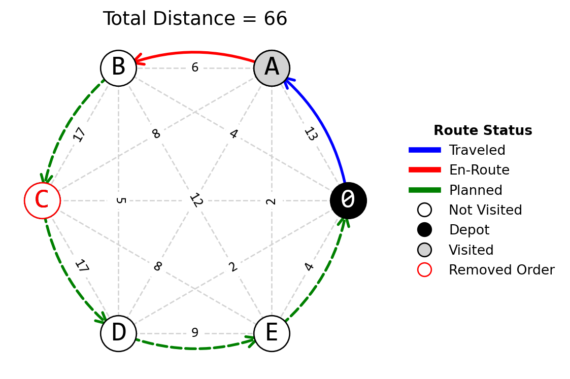
To calculate resilience, use the formula by Pant et al. (2014): \[ \mathcal{R}_{\varphi} (t_r|e_j) = \frac{[\varphi(t_r|e_j) - \varphi(t_d|e_j)]}{[\varphi(t_0) - \varphi(t_d|e_j)]} \ \ \ \forall e_j \in \mathcal{D} \]
Where:
- \(t_0\) is the initial time before the disruption.
- \(t_d\) is the time at disruption.
- \(t_r\) is the time of recovery to be evaluated.
- \(\varphi(t_0)\) is the system service function at initial time \(t_0\).
- \(\varphi(t_d|e_j)\) is the system service function at the time of disruption due to event \(e_j\).
- \(\varphi(t_r|e_j)\) is the system service function at the time of recovery being evaluated due to event \(e_j\).
- \(\mathcal{D}\) is the set of all disruptive events considered.
Answer
Reoptimization After Customer Removal (Solution). To reoptimize the path considering that customer C has canceled the order, and each served customer provides a benefit of 15, you will need to update the path to exclude C and calculate the new profit.
The original path was (0→A→B→C→D→E→0) and you’re currently on the way to B. After serving B, since C has canceled, the new path constructed using the nearest neighbor algorithm is (0→A→B→D→E→0).
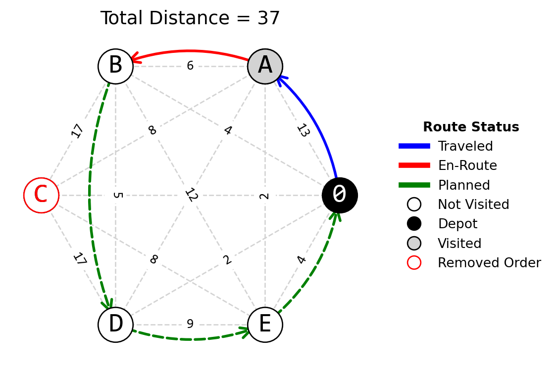
To quantify resilience in this context, we would consider the original state (serving all customers), the disrupted state (C canceling the order), and the recovered state (the new route without C).
- Original state profit = Original benefit (5 \(\times\) 15 = 75) - Original route cost (66) = 9
- Disrupted state profit = Original profit (5 \(\times\) 15 - 66 = 9 ) - Benefit from C (15) = -6
- Recovered state profit = New benefit (4 \(\times\) 15 = 60) - new route cost (37) = 23
Using the formula for resilience where \(\varphi(t_0)\) is the original state profit, \(\varphi(t_d|e_j)\) is the disrupted state profit, and \(\varphi(t_r|e_j)\) is the recovered state profit:
\[\mathcal{R}_{\varphi} (t_r|e_j) = \frac{[\varphi(t_r|e_j) - \varphi(t_d|e_j)]}{[\varphi(t_0) - \varphi(t_d|e_j)]}\]
\[\mathcal{R}_{\varphi} (t_r|e_j) = \frac{[(23) - (-6)]}{[(9) - (-6)]} = \frac{[29]}{[(15)]} = 1.93\]
The resilience of the reoptimized approach, given the disruption of removing a customer C, is approximately 1.93.
The resilience value, in this context, measures how effectively the reoptimized route recovers from the disruption, which in this scenario is the removal of customer C.
The resilience value is calculated on a scale where:
- A value of 1 would imply a perfect recovery, where the reoptimized system is as cost-efficient as the original system before the disruption occurred (e.g., the route is adjusted seamlessly without the canceled customer, maintaining the original efficiency or profit).
- A value of 0 would indicate no recovery benefit from reoptimization, where the disruption’s impact (i.e., the loss of the canceled customer’s benefit) is fully felt, and the reoptimized route offers no profit improvement over simply accepting the reduced number of customers.
- A value greater than 1 would suggest the reoptimized system is more cost-efficient than the original system (e.g., removing the customer from the route leads to significant savings in travel costs that outweigh the loss of their benefit, thus increasing overall profit).
- A negative value would indicate that the reoptimized system is performing worse than if the disruption hadn’t been managed, which in this context could mean the route adjustments lead to higher costs that do not justify the loss of the customer’s benefit (e.g., the reoptimization results in longer travel distances that outweigh the benefit of serving the remaining customers).
Exercise 9.3 (Reoptimization After Customer Insertion) Reoptimization After Customer Insertion. In the network shown in Figure 9.4, suppose a new customer E appears while you are en route to serve customer B. Reoptimization, if necessary, is conducted only after a customer has been served. Not serving this new customer incurs a cost of 15 to the company. The conversion between distance and cost is on a 1:1 basis. Design a reoptimization strategy using the nearest neighbor method to address this problem, and calculate the resilience of your approach based on the provided solution.
| To | 0 | A | B | C | D | E |
|---|---|---|---|---|---|---|
| From | ||||||
| 0 | 0 | 13 | 4 | 6 | 2 | 4 |
| A | 13 | 0 | 6 | 8 | 16 | 2 |
| B | 4 | 6 | 0 | 17 | 5 | 12 |
| C | 6 | 8 | 17 | 0 | 17 | 8 |
| D | 2 | 16 | 5 | 17 | 0 | 9 |
| E | 4 | 2 | 12 | 8 | 9 | 0 |
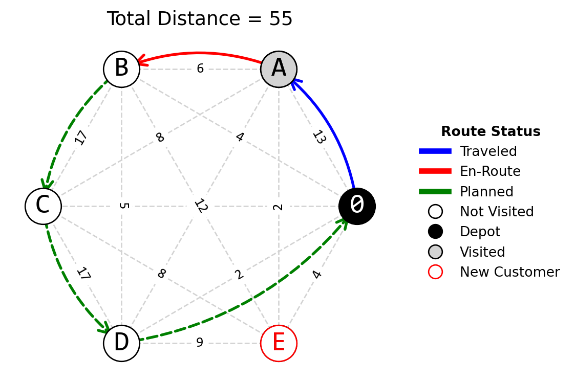
To calculate resilience, use the formula by Pant et al. (2014): \[ \mathcal{R}_{\varphi} (t_r|e_j) = \frac{[\varphi(t_r|e_j) - \varphi(t_d|e_j)]}{[\varphi(t_0) - \varphi(t_d|e_j)]} \ \ \ \forall e_j \in \mathcal{D} \]
Where:
- \(t_0\) is the initial time before the disruption.
- \(t_d\) is the time at disruption.
- \(t_r\) is the time of recovery to be evaluated.
- \(\varphi(t_0)\) is the system service function at initial time \(t_0\).
- \(\varphi(t_d|e_j)\) is the system service function at the time of disruption due to event \(e_j\).
- \(\varphi(t_r|e_j)\) is the system service function at the time of recovery being evaluated due to event \(e_j\).
- \(\mathcal{D}\) is the set of all disruptive events considered.
Answer
Reoptimization After Customer Insertion (Solution). Given the original state of the path as (0→A→B→C→D→0) and the reoptimized path accounting for the new customer E, we should follow these steps:
- Serve customer B as planned.
- Reoptimize the path considering customer E’s addition and using the nearest neighbor method from B, leading to the new route (0→A→B→D→E→C→0).
The total cost for the original plan (0→A→B→C→D→0) is 55, and the total cost for the reoptimized path (0→A→B→D→E→C→0) is 47.
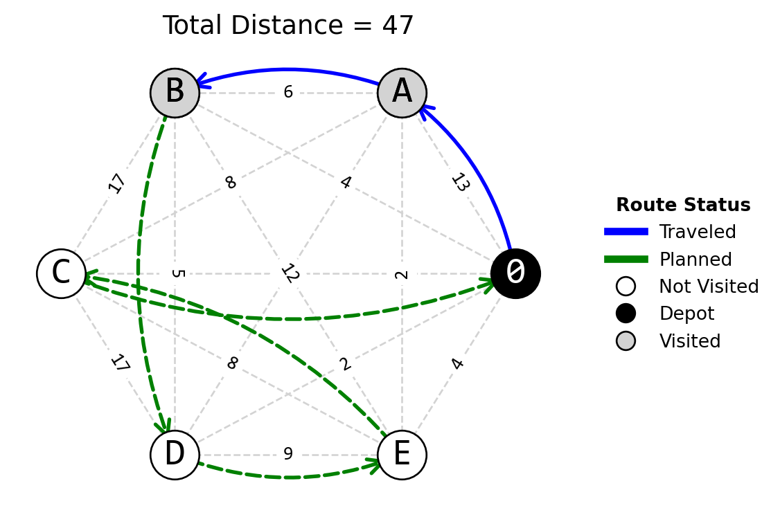
Considering the original state is the original plan, the disrupted state to be the point where we must decide whether to add E to the path (with the penalty cost of 15), and the recovered state to be after E is added and the path is reoptimized (with cost 47).
The disrupted state cost includes the original path cost plus the penalty for not serving E, which would be 55 + 15 = 70.
Using the formula for resilience (Pant et al. 2014) where \(\varphi(t_0)\) is the cost of the original path, \(\varphi(t_d|e_j)\) is the disrupted state cost, and \(\varphi(t_r|e_j)\) is the recovered state cost:
\[\mathcal{R}_{\varphi} (t_r|e_j) = \frac{[\varphi(t_r|e_j) - \varphi(t_d|e_j)]}{[\varphi(t_0) - \varphi(t_d|e_j)]}\]
\[\mathcal{R}_{\varphi} (t_r|e_j) = \frac{[47 - 70]}{[55 - 70]} = \frac{[-23]}{[-15]} = 1.53\]
The resilience of the reoptimized approach, given the disruption of adding customer E, is approximately 1.53.
The resilience value, in this context, measures how effectively the reoptimized route recovers from the disruption, which in this scenario is the addition of customer E.
The resilience value is calculated on a scale where:
- A value of 1 would imply a perfect recovery, where the reoptimized system is as cost-efficient as the original system before the disruption occurred (e.g., the new customer was incorporated into the route without any additional travel distance).
- A value of 0 would indicate no recovery benefit from reoptimization, where the disruption’s impact (i.e., detouring) is as detrimental as not serving the new customer at all (and incurring the full penalty cost).
- A value greater than 1 would suggest the reoptimized system is more cost-efficient than the original system (e.g., servicing the new customer leads to a more efficient path through other customers).
- A negative value would indicate that the reoptimized system is performing even worse than if it had just absorbed the penalty cost (e.g., the distance travelled to serve the new customer is too high).
Exercise 9.4 (VND Binary Truck Loading) VND Binary Truck Loading. Consider the following binary integer programming problem that represents a truck loading scenario, where the goal is to maximize the profit of the loaded items without exceeding the truck’s weight capacity:
Maximize the total profit of the items selected for loading:
\[18x_1 + 15x_2 + 35x_3 + 25x_4 + 19x_5 + 10x_6 + 40x_7 + 30x_8\]
Subject to the weight capacity of the truck:
\[6x_1 + 4x_2 + 7x_3 + 4x_4 + 5x_5 + 3x_6 + 10x_7 + 8x_8 \leq 30\]
Where the decision variables \(x_i\) indicate whether item \(i\) is loaded (1) or not (0), for \(i = 1, 2, ..., 8\).
Given this problem:
- Propose an initial solution heuristic that would provide a starting solution for a Variable Neighborhood Descent (VND) algorithm. Describe how you would prioritize item selection and how you would determine the initial configuration of loaded items.
- Define two distinct neighborhood structures to explore different combinations of loaded items that could potentially increase the total profit while adhering to the weight constraint.
- Apply the VND algorithm for 5 iterations, using the initial solution and neighborhood structures proposed. Detail each iteration step, including how the solution changes and the decision-making process for when to switch between neighborhood structures.
Remember to clarify the neighborhood structures with examples. The iterations should illustrate the process of searching for an improved solution, switching between neighborhoods when the current neighborhood does not yield further improvement, and halting the algorithm after the predetermined number of iterations or when no further improvement can be found.
Answer
VND Binary Truck Loading (Hint).
A viable heuristic for loading the truck would be to prioritize items by their profit, loading them in descending order of profitability until the truck’s capacity is fully utilized. For instance, an initial solution where the truck is loaded with items 3, 4, 7, and 8 (indicated by the binary sequence
0 0 1 1 0 0 1 1) results in an objective (profit) value of 130.Two potential neighborhood structures to consider are:
- Exchange an item on the truck with one not currently loaded.
- Identify two items currently loaded on the truck and swap each with an item not loaded.
Both 1. and 2. movements are valid only if the truck capacity is not exceed.
The procedure for the Variable Neighborhood Descent (VND) algorithm is as follows:
- Step 1: Begin with the initial solution and iteratively apply local search using the first neighborhood structure until no further improvements can be made.
- Step 2: If the first neighborhood fails to yield a better solution, maintain the current solution and apply local search using the second neighborhood structure.
- Step 3: Should the second neighborhood lead to an improved solution, revert to Step 1 with this new, improved solution.
- Step 4: If there are no improvements with the second neighborhood, conclude the algorithm.
Algorithmically (Gendreau and Potvin 2019):
- Input:
- \(x\): Initial solution.
- \(k_{\text{max}}\): Number of neighborhood structures \(N_k\). Each neighborhood \(N_k\) is characterized by a specific strategy for exploring the solution space around \(x\).
- Output: Local minimum w.r.t. all \(k_{\text{max}}\) neighborhoods.
- Procedure:
- Initialize \(k\) to 1
- Repeat until \(k = k_{\text{max}}\):
- \(x' \gets \text{arg min}_{y \in N_k(x)} f(y)\) (Find the best neighbor in \(N_k(x)\))
- If \(f(x') < f(x)\) then
- \(x \gets x'\) (Update incumbent)
- Reset \(k\) to 1 (Initial neighborhood)
- Else
- Increment \(k\) (Next neighborhood)
- Return \(x\)