3  Mathematical Modeling with Python

This tutorial provides a hands-on approach to understanding and implementing mathematical models in Python. It consolidates the legacy root tutorial tlm_tutorial_02_math_modeling_with_python.qmd.

3.1 Instructions

Along with this tutorial, some Tasks activities are proposed. Self-assess if you can solve them on your own.

3.2 Prerequisites

In this tutorial, we will use gurobipy, numpy, pandas, and folium.

You can install each package using the following command in your terminal or command prompt:

pip install name_of_package

For example, to install pandas, you would use:

pip install pandas

Repeat this process for numpy, pandas, gurobipy, and folium.

In notebooks, you can install packages using the %pip magic command:

%pip install name_of_package

Below, we install the packages we will use in this tutorial (assuming we are in a Jupyter notebook):

# Packages for data manipulation
%pip install -q pandas  # '-q' installs quietly (no output)
%pip install -q numpy

# Packages for optimization
%pip install -q gurobipy

# Packages for data visualization
%pip install -q folium
%pip install -q matplotlib
%pip install -q seaborn

# The '-q' (quiet) flag suppresses most output from pip.
# This is useful in notebooks to keep the output clean.
# You can use '-qq' for even less output, but errors/warnings may be hidden.

You can install these in the terminal using:

pip install gurobipy numpy pandas folium matplotlib seaborn

3.3 NumPy Arrays and Vectorization

When dealing with large-scale, complex programs, computational efficiency becomes crucial. This efficiency depends on various factors, such as the size and complexity of your program and the nature of the problems you’re addressing.

Consider a scenario where you need to add a number to a list:

Code
from time import time

start_time = time()

# Creating a list of 50,000,000 elements
num_list = [*range(0, 50000000)]
for i in range(len(num_list)):
    num_list[i] += 1

end_time = time()
elapsed_time = end_time - start_time
print("Elapsed time:", elapsed_time)
Elapsed time: 4.760638236999512

Here, we measure the time taken to perform the operations. Using a timer is essential for gauging the efficiency of your algorithm. Timing is not the only way to measure performance. You can also estimate performance by counting the number of operations (algorithmic complexity). Further reading on performance measurement with Python can be found here.

The time taken by the above program might give the impression of efficiency, but imagine needing to run this multiple times within a larger codebase. This is where performance optimization becomes crucial.

NoteTask

Why is restricting a list to only one type of data beneficial for computational efficiency?

Enter NumPy, a core library for scientific computing in Python. It adds data structures and tools for a wide range of mathematical operations. NumPy arrays are similar to lists, but they offer key performance advantages:

Code
import numpy as np

normal_list = [0, 1, 2, 3, 4, 5]
print("Normal List:", normal_list)

# Creating a NumPy array from the normal list
num_array = np.array(normal_list)
print("NumPy Array:", num_array)

# Adding 1 to each element of the NumPy array
num_array += 1
print("Updated NumPy Array:", num_array)
Normal List: [0, 1, 2, 3, 4, 5]
NumPy Array: [0 1 2 3 4 5]
Updated NumPy Array: [1 2 3 4 5 6]

NumPy’s array function is versatile, accepting various forms of input, like Python lists. A noticeable difference is the absence of commas in the printed NumPy array. Beyond aesthetics, the key advantage of NumPy arrays is their support for vector operations, allowing for simultaneous and fast mathematical manipulations.

Another difference is how lists and arrays handle modifications: lists require element-wise changes, whereas arrays can update all elements in one operation.

Code
start_time = time()
num_array = np.arange(0, 50000000)

# Adding 1 to each element of the NumPy array
num_array += 1
end_time = time()

elapsed = end_time - start_time
print("Elapsed time with NumPy:", elapsed)
Elapsed time with NumPy: 0.16316485404968262

np.arange, similar to range, generates a NumPy array. The speedup from using NumPy arrays over lists is significant for even simple operations. NumPy offers many other functions that utilize NumPy arrays as their foundational data structure.

Working with Matrices in NumPy

NumPy provides various ways to define and manipulate multi-dimensional arrays:

Code
# Define a 3x4 matrix
rows, columns = 3, 4
matrix_a = [[x for x in range(columns)] for x in range(rows)]
matrix_c = np.array(matrix_a)

# Define a 3x4 matrix using NumPy
matrix_b = np.arange(rows * columns).reshape(rows, columns)

print("Matrix A:", matrix_a)
print("Matrix C (NumPy):", matrix_c)
print("Matrix B (NumPy):", matrix_b)
Matrix A: [[0, 1, 2, 3], [0, 1, 2, 3], [0, 1, 2, 3]]
Matrix C (NumPy): [[0 1 2 3]
 [0 1 2 3]
 [0 1 2 3]]
Matrix B (NumPy): [[ 0  1  2  3]
 [ 4  5  6  7]
 [ 8  9 10 11]]

To examine the shape or dimensions of a NumPy array:

Code
print("Shape of Matrix B:", matrix_b.shape)
rows, cols = matrix_b.shape
print(f"Rows: {rows}, Columns: {cols}")
Shape of Matrix B: (3, 4)
Rows: 3, Columns: 4

Accessing specific elements:

Code
# Accessing an element at row 3, column 2
print("Element at row 3, column 2:", matrix_b[2][1])
Element at row 3, column 2: 9

Creating matrices with predefined values:

Code
# Creating a 2x2 zero-valued matrix
zero_matrix = np.zeros((2, 2), dtype=int)
print("Type of elements in zero_matrix:", type(zero_matrix[0][0]))

# Creating a 2x2 matrix with random values
random_matrix = np.random.random((2, 2))
print("Random Matrix:", random_matrix)
Type of elements in zero_matrix: <class 'numpy.int64'>
Random Matrix: [[0.39456319 0.49362522]
 [0.04999891 0.5243953 ]]
NoteTask

Create a large list (e.g., 7005 elements) of random numbers (1 to 7004) and compute the square root of each element using a loop. Compare this with the performance of a NumPy array and the np.sqrt function for vectorized operations. Measure the time taken and identify the fastest approach.

3.4 Reading and Writing Text Files

In scientific computing, manually entering data can be time-consuming and limited. Collected data is often saved to files for later retrieval in Python. Sometimes, data is stored in formats that are not straightforward to read, but Python libraries can help. In other cases, you may need manufacturers’ software to export the data into simpler formats like CSV or plain text files.

Reading from Files

The basic method to read a text file in Python is using the open function. This function returns an iterable file object, allowing you to iterate over each line using a for loop. For example, to read a simple data file with a single column of numbers, you might use:

Code
import numpy as np

input_file = open("data/raw/depot_id_list.txt", 'r')
data_list = []

for line in input_file:
    data_list.append(int(line))

input_file.close()
depots = np.array(data_list[:3], dtype=int)
print(depots)
[100 200 300]

Opening the file with open along with the argument 'r' means that the file is in read-only mode. It’s important to note that the data read from the file is initially in string format. For numerical operations, you need to convert it to the appropriate data type (e.g., int, float).

NoteTask

What happens if you remove int() from the program above and only append line?

Closing the file object after reading is good practice, especially to prevent potential file access issues later.

NoteTask

Why is closing the file a good practice? Give an example.

Pythonic Code Style

Pythonic code is characterized by being clear, concise, and maintainable. The example below demonstrates a Pythonic approach to reading files:

Code
data_list = []
with open("data/raw/depot_id_list.txt", 'r') as input_file:
    for line in input_file:
        data_list.append(int(line))
print(data_list)
[100, 200, 300, 400, 500]

This code uses the with statement, ensuring that the file is properly closed after the operations within the indented block are completed.

NoteTask

Extract the data from file att48.tsp and print the numbers to the screen.

Writing to Files

Writing to files is similar to reading them, but you open the file in write mode ('w'):

Code
new_data = [4, 5, 6, 7]
with open("data/processed/newFile.txt", 'w') as output_file:
    for number in new_data:
        output_file.write(str(number) + "\n")

This code writes to a file, creating it if it doesn’t exist or overwriting it if it does. To append data instead of overwriting, use append mode ('a'). Remember to convert non-string data to strings before writing, and use \n to add new lines after each entry.

Advanced File Operations

You can read and process files in various ways depending on your needs. Let’s consider the file att48.tsp, which contains a mix of text and numerical data. The contents of this file are:

NAME : att48 (http://elib.zib.de/pub/mp-testdata/tsp/tsplib/tsp/index.html)
COMMENT : 48 capitals of the US (Padberg/Rinaldi)
TYPE : TSP
DIMENSION : 48
EDGE_WEIGHT_TYPE : ATT
NODE_COORD_SECTION
1 6734 1453
2 2233 10
3 5530 1424
4 401 841
5 3082 1644
6 7608 4458
7 7573 3716
8 7265 1268
9 6898 1885
10 1112 2049
11 5468 2606
12 5989 2873
13 4706 2674
14 4612 2035
15 6347 2683
16 6107 669
17 7611 5184
18 7462 3590
19 7732 4723
20 5900 3561
21 4483 3369
22 6101 1110
23 5199 2182
24 1633 2809
25 4307 2322
26 675 1006
27 7555 4819
28 7541 3981
29 3177 756
30 7352 4506
31 7545 2801
32 3245 3305
33 6426 3173
34 4608 1198
35 23 2216
36 7248 3779
37 7762 4595
38 7392 2244
39 3484 2829
40 6271 2135
41 4985 140
42 1916 1569
43 7280 4899
44 7509 3239
45 10 2676
46 6807 2993
47 5185 3258
48 3023 1942

You can read this file line by line using the open function and process the data as needed:

Code
import numpy as np

# Initialize empty lists
c = []
d = []

# Open file in read mode
with open('data/raw/att48.tsp') as f:
    # Read all lines from file
    lines = f.readlines()

    # Split the 6th line for node_id, x, y headers
    node_id_header, x_header, y_header = lines[5].split("_")

    # Process each line starting from 7th line
    for line in lines[6:]:

        # Convert line to numpy array of integers
        b = np.fromstring(line, dtype=int, sep=' ')

        # Append array as list to 'c'
        c.append(b.tolist())

        # Split line, convert to int, append to 'd'
        d.append([int(num) for num in line.split()])

print("Headers:", node_id_header, x_header, y_header)
print(f"Data read using `np.fromstring` (shape = {len(c), len(c[0])}): {c}")
print(f"Data read using `split()`(shape = {len(c), len(c[0])}): {d}")
# Output second element of first list in 'c'
print(c[0][1])
# Output type of second element of first list in 'd'
print(type(d[0][1]))
Headers: NODE COORD SECTION

Data read using `np.fromstring` (shape = (48, 3)): [[1, 6734, 1453], [2, 2233, 10], [3, 5530, 1424], [4, 401, 841], [5, 3082, 1644], [6, 7608, 4458], [7, 7573, 3716], [8, 7265, 1268], [9, 6898, 1885], [10, 1112, 2049], [11, 5468, 2606], [12, 5989, 2873], [13, 4706, 2674], [14, 4612, 2035], [15, 6347, 2683], [16, 6107, 669], [17, 7611, 5184], [18, 7462, 3590], [19, 7732, 4723], [20, 5900, 3561], [21, 4483, 3369], [22, 6101, 1110], [23, 5199, 2182], [24, 1633, 2809], [25, 4307, 2322], [26, 675, 1006], [27, 7555, 4819], [28, 7541, 3981], [29, 3177, 756], [30, 7352, 4506], [31, 7545, 2801], [32, 3245, 3305], [33, 6426, 3173], [34, 4608, 1198], [35, 23, 2216], [36, 7248, 3779], [37, 7762, 4595], [38, 7392, 2244], [39, 3484, 2829], [40, 6271, 2135], [41, 4985, 140], [42, 1916, 1569], [43, 7280, 4899], [44, 7509, 3239], [45, 10, 2676], [46, 6807, 2993], [47, 5185, 3258], [48, 3023, 1942]]
Data read using `split()`(shape = (48, 3)): [[1, 6734, 1453], [2, 2233, 10], [3, 5530, 1424], [4, 401, 841], [5, 3082, 1644], [6, 7608, 4458], [7, 7573, 3716], [8, 7265, 1268], [9, 6898, 1885], [10, 1112, 2049], [11, 5468, 2606], [12, 5989, 2873], [13, 4706, 2674], [14, 4612, 2035], [15, 6347, 2683], [16, 6107, 669], [17, 7611, 5184], [18, 7462, 3590], [19, 7732, 4723], [20, 5900, 3561], [21, 4483, 3369], [22, 6101, 1110], [23, 5199, 2182], [24, 1633, 2809], [25, 4307, 2322], [26, 675, 1006], [27, 7555, 4819], [28, 7541, 3981], [29, 3177, 756], [30, 7352, 4506], [31, 7545, 2801], [32, 3245, 3305], [33, 6426, 3173], [34, 4608, 1198], [35, 23, 2216], [36, 7248, 3779], [37, 7762, 4595], [38, 7392, 2244], [39, 3484, 2829], [40, 6271, 2135], [41, 4985, 140], [42, 1916, 1569], [43, 7280, 4899], [44, 7509, 3239], [45, 10, 2676], [46, 6807, 2993], [47, 5185, 3258], [48, 3023, 1942]]
6734
<class 'int'>
In this example, data is read line by line and transformed into numeric values. The np.fromstring method is used to convert string data to numbers, based on the specified data type (dtype=int). Be aware that converting lists to arrays may not work as expected with irregularly sized data.

The output above may be wide and hard to read. Use pretty-printing and a short preview to improve readability:

Code
from pprint import pprint # Importing pprint for better readability of output

pprint(c)
[[1, 6734, 1453],
 [2, 2233, 10],
 [3, 5530, 1424],
 [4, 401, 841],
 [5, 3082, 1644],
 [6, 7608, 4458],
 [7, 7573, 3716],
 [8, 7265, 1268],
 [9, 6898, 1885],
 [10, 1112, 2049],
 [11, 5468, 2606],
 [12, 5989, 2873],
 [13, 4706, 2674],
 [14, 4612, 2035],
 [15, 6347, 2683],
 [16, 6107, 669],
 [17, 7611, 5184],
 [18, 7462, 3590],
 [19, 7732, 4723],
 [20, 5900, 3561],
 [21, 4483, 3369],
 [22, 6101, 1110],
 [23, 5199, 2182],
 [24, 1633, 2809],
 [25, 4307, 2322],
 [26, 675, 1006],
 [27, 7555, 4819],
 [28, 7541, 3981],
 [29, 3177, 756],
 [30, 7352, 4506],
 [31, 7545, 2801],
 [32, 3245, 3305],
 [33, 6426, 3173],
 [34, 4608, 1198],
 [35, 23, 2216],
 [36, 7248, 3779],
 [37, 7762, 4595],
 [38, 7392, 2244],
 [39, 3484, 2829],
 [40, 6271, 2135],
 [41, 4985, 140],
 [42, 1916, 1569],
 [43, 7280, 4899],
 [44, 7509, 3239],
 [45, 10, 2676],
 [46, 6807, 2993],
 [47, 5185, 3258],
 [48, 3023, 1942]]
ImportantTask

Create a program that reads a distance matrix in kilometers from a file and converts it into a time matrix in seconds, assuming an average speed. The program should read the distance matrix from a file named distance_matrix.txt, where distances are given in kilometers. Assume an average speed of 60 km/h for the conversion. After converting the distances to time in seconds, the program should save the resulting matrix to a file named time_matrix.txt.

3.5 Loading Data Using NumPy

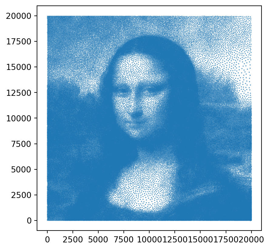
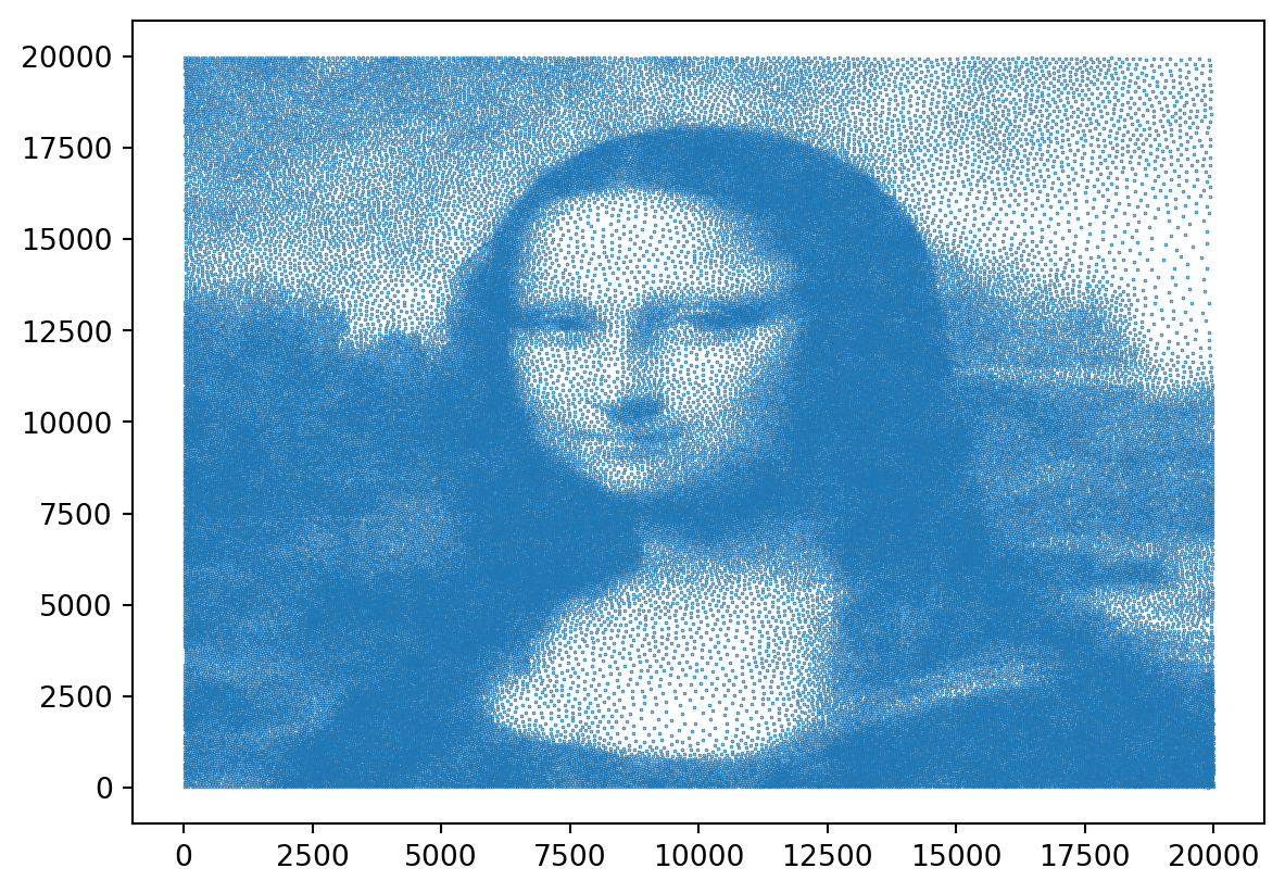
NumPy’s loadtxt function is useful for reading grid-formatted text data into a NumPy array. Here, we use matplotlib for plotting the data:

Code
import numpy as np
import matplotlib.pyplot as plt

# Load data from "mona-lisa100K.tsp" file
# Assuming the data is separated by spaces and is of integer type
input_array = np.loadtxt("data/raw/mona-lisa100K.tsp", dtype="i", delimiter=' ')

# Transpose the input array for easier data manipulation
transposed = input_array.transpose()

# Print the original and transposed arrays to the console
print("Original Array:\n", input_array)
print("Transposed Array:\n", transposed)

# Extracting individual arrays from the transposed array
# First row (IDs), second row (X coordinates), third row (Y coordinates)
ids = transposed[0]
x_data = transposed[1]
y_data = transposed[2]

# Plotting the data using a scatter plot
# 's=0.1' sets the size of each point in the plot
plt.scatter(x_data, y_data, s=0.1)

# Set equal scaling for both axes (otherwise, the image may appear distorted)
plt.gca().set_aspect('equal', adjustable='box')

# Display the scatter plot
plt.show()
Original Array:
 [[     1  14991   8390]
 [     2  13616  12541]
 [     3    961  10768]
 ...
 [ 99998  10567  17917]
 [ 99999  10666    665]
 [100000  13425   1002]]
Transposed Array:
 [[     1      2      3 ...  99998  99999 100000]
 [ 14991  13616    961 ...  10567  10666  13425]
 [  8390  12541  10768 ...  17917    665   1002]]

In this example, the dtype parameter is set to 'i', indicating that the elements are loaded as integers (check other types here). To inspect the types of elements in the array, you can use the dtype attribute of the array:

Code
print(input_array.dtype)
int32

When the parameter unpack is set to True, the columns in the data are unpacked into separate arrays. In the example, the first column of the data is assigned to ids, the second column to x_data, and the third column to y_data. If unpack is not set, or is set to False, the data is read into a single 2D array.

Code
import numpy as np
import matplotlib.pyplot as plt

# Using unpack to directly separate the data columns
ids, x_data, y_data = np.loadtxt(
    "data/raw/mona-lisa100K.tsp",
    dtype="i",
    delimiter=' ',
    unpack=True)

# Plotting the data using a scatter plot
# 's=0.1' sets the size of each point in the plot
plt.scatter(x_data, y_data, s=0.1)

# Display the scatter plot
plt.show()

The beginning of some files may have metadata that should be ignored. Using skiprows allows you to skip a specified number of lines. For instance, skiprows=6 will skip the first six lines of the file:

Code
import numpy as np
import matplotlib.pyplot as plt


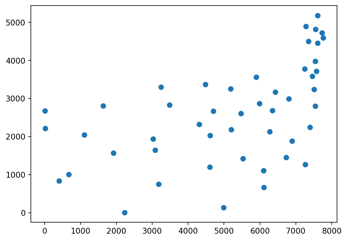
ids, x_data, y_data = np.loadtxt("data/raw/att48.tsp", dtype="i", delimiter=' ', unpack=True, skiprows=6)

plt.scatter(x_data, y_data)

# Display the scatter plot
plt.show()

It’s important to note that loadtxt is primarily designed to handle numerical data. If the file contains a mix of text and numbers, or if the data is not neatly arranged in a grid format, loadtxt may not be the best tool for the job. In such cases, a combination of Python’s file reading capabilities and list manipulation can be used to process the data.

NoteTask

Create a program that reads mona-lisa100K.tsp using loadtxt and plots only the odd rows.

3.6 Saving Data Using NumPy

Saving NumPy array data can be performed using the savetxt function:

Code
data_to_save = np.array([[1, 2], [2, 3], [3, 7]])

np.savetxt("data/processed/output.txt", data_to_save)
ImportantTask

Write a program that reads the coordinate data from the file mona-lisa100K.tsp, which represents an artistic depiction of the Mona Lisa. Use np.loadtxt to load the coordinate data. Your task is to invert the positions of the coordinates, effectively creating a mirrored image of the original artwork. This will involve swapping the x and y coordinates of each point. Once the coordinates are inverted, use matplotlib to plot both the original and the inverted images side by side for visual comparison. Finally, save the inverted coordinates to a new file named inverted-mona-lisa100K.tsp using np.savetxt.

3.7 Data Visualization

Python offers various packages for generating graphs and plots, with Matplotlib being one of the best known. Matplotlib excels at creating publication-quality figures and, despite its steep learning curve, offers more customization than software like Excel. Once mastered, a set of personal plot templates can be reused and modified throughout your professional career.

Histograms

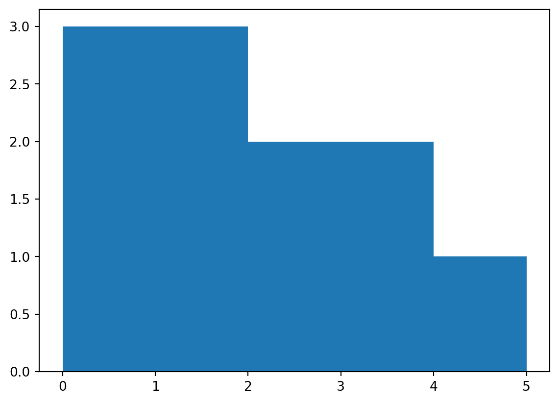
The code below imports Matplotlib and plots a histogram of a given list of numbers.

Code
import matplotlib.pyplot as plt

# Generating a list of numbers
list_of_numbers = [0.2, 0.3, 0.2, 1.2, 1.7, 1.4, 2.1, 2.5, 3.1, 3.22, 4.6, 5.1]

# Plotting a histogram with specified bins
plt.hist(list_of_numbers, bins=[0, 1, 2, 3, 4, 5])

# Displaying the histogram
plt.show()

NoteTask

Explore the function of bins in the histogram. What happens if it is removed?

NoteTask

Generate 505 random numbers between 1 and 7, plot them in a histogram, and observe the distribution.

Line Plots

Line plots can be created similarly to histograms:

Code
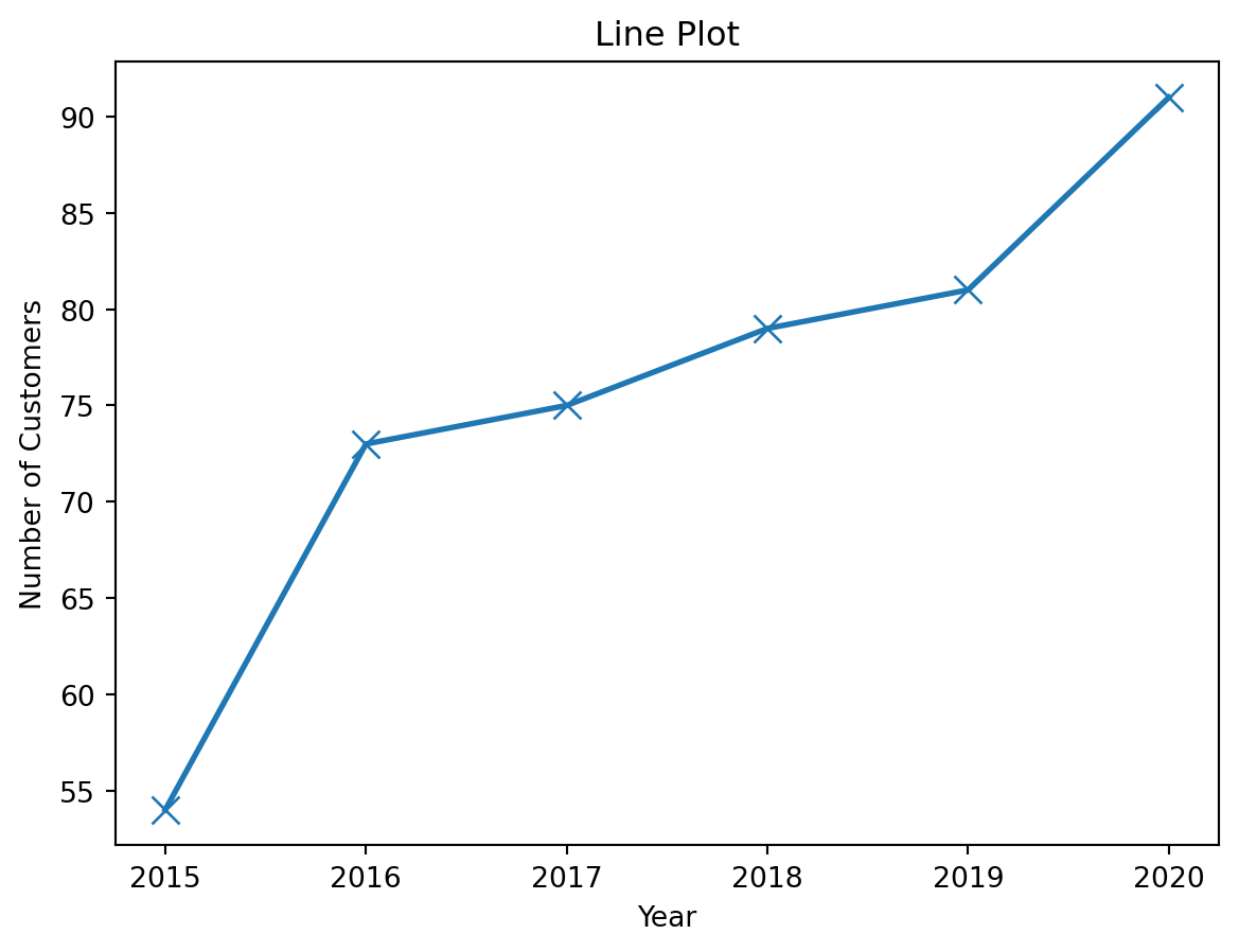
x_data = [2015, 2016, 2017, 2018, 2019, 2020]
y_data = [54, 73, 75, 79, 81, 91]

# Creating a line plot with customizations
plt.plot(x_data, y_data, linestyle="-", marker="x", markersize=10, linewidth=2)
plt.title("Line Plot")
plt.xlabel("Year")
plt.ylabel("Number of Customers")

# Saving the plot to a PDF file
from pathlib import Path

base_dir = Path("tutorials/tlm_tutorial_intro_math_programming")
if not base_dir.exists():
    base_dir = Path(".")

output_dir = base_dir / "data" / "plots"
output_dir.mkdir(parents=True, exist_ok=True)
plt.savefig(output_dir / "customersGrow.pdf")

# Displaying the plot
plt.show()

For more details on the plot function, including options for colors, markers, and line types, refer to the Matplotlib documentation.

NoteTask

Modify the axis range of the plot to display values from 0 to 10. Use online resources to find the correct syntax.

Exploring Alternatives

When it comes to data visualization in Python, several libraries offer diverse functionalities beyond the well-known Matplotlib. Among these, Seaborn, Plotly, and Folium stand out for their unique features and use cases.

  • Seaborn: An extension to Matplotlib, Seaborn simplifies the creation of attractive and informative statistical graphics (Seaborn Documentation).
  • Plotly: This library specializes in interactive and aesthetically pleasing visualizations and is particularly useful for web-based dashboards (Plotly Python Graphing Library).
  • Folium: Ideal for geographical data, Folium leverages the capabilities of Leaflet.js to create interactive maps with ease (Folium Documentation).

Tip: Creating Charts Using AI (ChatGPT)

One innovative approach to data visualization is leveraging AI, like ChatGPT, to assist in creating and brainstorming complex charts. For instance, you can describe your dataset and requirements to ChatGPT, and it can suggest the most suitable types of visualizations, provide code snippets, or even help troubleshoot issues with your visualization code.

Example

The following code snippet demonstrates how to create an interactive map using Folium, showing the locations of US state capitals:

Code
import pandas as pd
import folium

# Load US state capitals data from a CSV file
capitals = pd.read_csv("data/raw/us-state-capitals.csv")

# Initialize a Folium map centered on the geographical center of the USA
# Set initial zoom level and map style (tiles)
m = folium.Map(location=[39.8283, -98.5795], zoom_start=4, tiles="cartodb positron")

# Iterate through the DataFrame and add a marker for each capital
for idx, row in capitals.iterrows():
    folium.Marker(
        location=[row['latitude'], row['longitude']],
        popup=row['name'],  # Display the name of the capital on marker click
    ).add_to(m)

# Display the interactive map in the notebook
m
Make this Notebook Trusted to load map: File -> Trust Notebook

In this code:

  • Folium is installed and imported, alongside pandas for data handling.
  • A CSV file containing data of US state capitals is loaded into a pandas DataFrame.
  • A Folium map object is created, centered around the central coordinates of the USA.
  • The script iterates through the capitals DataFrame, adding a marker on the map for each capital using its latitude and longitude.
  • The map is displayed with interactive markers, each showing the name of the corresponding state capital upon clicking.

3.8 Solving Mathematical Models with Python

Solving mathematical models in Python can be achieved using various libraries and solvers.

Solvers

Solvers are tools that find the optimal solution to a mathematical problem, such as linear programming, mixed-integer programming, or quadratic programming. Common solvers include:

  • CBC: An open-source mixed integer programming (MIP) solver.
  • CPLEX: A high-performance solver for large-scale linear, mixed-integer, and quadratic programming.
  • Gurobi: Known for its performance and robustness in solving MIPs, linear, and quadratic programming problems.

Both CPLEX and Gurobi are commercial solvers, but they offer free academic licenses.

Connecting Solvers to Python with Open-Source Libraries

Libraries offer a unified interface for formulating mathematical problems using a consistent modeling syntax. One of the significant advantages is their ability to interface with a variety of solvers, both free and commercial, allowing the same model to be solved by different algorithms without altering the fundamental model structure. Examples of Python libraries include:

  • PuLP: Integrates with several solvers, including CPLEX and Gurobi, and can automatically call these solvers to solve the defined model.
  • Pyomo: An open-source tool that can interface with numerous solvers, including CPLEX and Gurobi. Pyomo models need to specify the solver before solving.

Connecting Solvers Directly to Python with APIs

Some solvers, like Gurobi, have their own Python APIs, allowing direct interaction with the solver without an intermediary library. This can be beneficial for advanced users who require more control over solver behavior. For example, if you need to set specific solver parameters or access advanced features, using the solver’s Python API directly might be the best approach. This is why we adopt gurobipy (Gurobi’s Python API) in this course.

3.9 Example: Solving the TSP with Gurobi

Let’s adapt the Traveling Salesman Problem (TSP) solution to use Gurobi. TSP aims to find the shortest tour that visits all cities exactly once and returns to the origin city.

Installing Gurobi

Before using Gurobi, it must be installed and activated with a valid license.

  1. Install Gurobi via pip:

    pip install gurobipy
  2. Obtain a License:

    • If you are an academic user, you can obtain a free license from Gurobi’s website.

    • After downloading, activate the license using:

      grbgetkey YOUR_LICENSE_KEY
  3. Verify the Installation: Run the following Python command to check if Gurobi is accessible:

    Code
    import gurobipy as gp
    print(gp.gurobi.version())
    (13, 0, 1)

    If the installation is successful, it will return the Gurobi version.

Steps to Model a Mathematical Program

When constructing a mathematical model in Python, it’s essential to consider various components of the model. These include:

  1. Importing the solver
  2. Retrieving the input parameters
  3. Defining the decision variables
  4. Adding the objective function
  5. Introducing the constraints
  6. Solving the model
  7. Printing out the output

In this section, we will focus on solving the Traveling Salesman Problem (TSP) using Gurobi.

The Traveling Salesman Problem (TSP)

The Traveling Salesman Problem (TSP) aims to find the shortest possible tour that visits each city exactly once and returns to the starting city. The distances between cities are represented by a distance matrix \(D\), where each element \(c_{i,j}\) denotes the distance from city i to city j.

Let \(n\) be the total number of cities in the problem. The goal is to find a sequence in which to visit these cities, minimizing the total travel cost while ensuring that every city is visited exactly once.

Mathematical Formulation

The TSP is formulated as follows:

  • Objective Function (Minimize the total distance):

    \[ \min \sum_{i \neq j} c_{i,j} \cdot x_{i,j} \]

    The objective function minimizes the total travel cost by summing the distances \(c_{i,j}\) for every selected route \(x_{i,j}\).

  • Constraints:

    • Each city must be left exactly once:

      \[ \sum_{j \neq i} x_{i,j} = 1, \quad \forall i \in \{1, \dots, n\} \]

    • Each city must be entered exactly once:

      \[ \sum_{i \neq j} x_{i,j} = 1, \quad \forall j \in \{1, \dots, n\} \]

    • Subtour elimination constraint (Miller-Tucker-Zemlin formulation):

      \[ u_i - u_j + n \cdot x_{i,j} \leq n - 1, \quad \forall i, j \in \{2, \dots, n\}, \quad i \neq j \]

  • Decision Variables:

    • \(x_{i,j} \in \{0,1\}\): Binary variable, indicating whether the route between city i and j is used.
    • \(u_i\): Continuous variable, representing the position of city i in the tour and used for subtour elimination.

This formulation ensures that all cities are visited exactly once, no city is skipped, and the solution forms a single tour instead of multiple disconnected loops.

Gurobi Implementation

Step 1: Load Data and Compute Distance Matrix

Code
import numpy as np
import math
import gurobipy as gp
from gurobipy import GRB
from pprint import pprint

# Load city coordinates from a file
cities = np.loadtxt(
    "data/raw/att48.tsp",
    dtype="i",
    delimiter=" ",
    skiprows=6,
    max_rows=5,  # Only using 5 cities for this example
)

# Function to compute Euclidean distance between two cities
def euclidean_distance(p1, p2):
    return math.sqrt((p1[0] - p2[0]) ** 2 + (p1[1] - p2[1]) ** 2)

# Construct the distance matrix
dist_matrix = np.array([
    [euclidean_distance((x_o, y_o), (x_d, y_d)) for _, x_d, y_d in cities]
    for _, x_o, y_o in cities
])

city_ids = [int(city[0]) for city in cities]
print("City IDs:", city_ids)
pprint(dist_matrix.round(2))  # Display the computed distances
City IDs: [1, 2, 3, 4, 5]
array([[   0.  , 4726.65, 1204.35, 6362.5 , 3656.99],
       [4726.65,    0.  , 3587.42, 2011.66, 1841.4 ],
       [1204.35, 3587.42,    0.  , 5162.03, 2457.87],
       [6362.5 , 2011.66, 5162.03,    0.  , 2798.67],
       [3656.99, 1841.4 , 2457.87, 2798.67,    0.  ]])

This code loads city coordinates from a file using NumPy’s loadtxt(), computes the Euclidean distances between cities, and stores them in a distance matrix. The matrix is printed for verification.

Step 2: Define Gurobi Model and Variables

Code
# Number of cities
n = len(cities)

# Create a new Gurobi model
model = gp.Model("TSP")

# Binary decision variables: x[i, j] = 1 if travel from i to j is selected
x = model.addVars(n, n, vtype=GRB.BINARY, name="x")

# Continuous subtour elimination variables
u = model.addVars(n, vtype=GRB.CONTINUOUS, lb=0, ub=n - 1, name="u")
Set parameter Username
Set parameter LicenseID to value 2777413
Academic license - for non-commercial use only - expires 2027-02-10

The variable $ n $ represents the total number of cities. The model initializes binary decision variables x[i, j] for selecting routes and continuous variables u[i] to store the position of each city in the tour. The u[i] variables help maintain a logical order of visits and prevent the solver from forming disjoint subtours.

If we print the variables, we can see the structure of the decision variables:

Code
# Update the model to display the decision variables
model.update()

# Display the decision variables x_ij
print("Decision Variables x:")
pprint(x)

# Display the decision variables u_i
print("\nDecision Variables u:")
pprint(u)
Decision Variables x:
{(0, 0): <gurobi.Var x[0,0]>,
 (0, 1): <gurobi.Var x[0,1]>,
 (0, 2): <gurobi.Var x[0,2]>,
 (0, 3): <gurobi.Var x[0,3]>,
 (0, 4): <gurobi.Var x[0,4]>,
 (1, 0): <gurobi.Var x[1,0]>,
 (1, 1): <gurobi.Var x[1,1]>,
 (1, 2): <gurobi.Var x[1,2]>,
 (1, 3): <gurobi.Var x[1,3]>,
 (1, 4): <gurobi.Var x[1,4]>,
 (2, 0): <gurobi.Var x[2,0]>,
 (2, 1): <gurobi.Var x[2,1]>,
 (2, 2): <gurobi.Var x[2,2]>,
 (2, 3): <gurobi.Var x[2,3]>,
 (2, 4): <gurobi.Var x[2,4]>,
 (3, 0): <gurobi.Var x[3,0]>,
 (3, 1): <gurobi.Var x[3,1]>,
 (3, 2): <gurobi.Var x[3,2]>,
 (3, 3): <gurobi.Var x[3,3]>,
 (3, 4): <gurobi.Var x[3,4]>,
 (4, 0): <gurobi.Var x[4,0]>,
 (4, 1): <gurobi.Var x[4,1]>,
 (4, 2): <gurobi.Var x[4,2]>,
 (4, 3): <gurobi.Var x[4,3]>,
 (4, 4): <gurobi.Var x[4,4]>}

Decision Variables u:
{0: <gurobi.Var u[0]>,
 1: <gurobi.Var u[1]>,
 2: <gurobi.Var u[2]>,
 3: <gurobi.Var u[3]>,
 4: <gurobi.Var u[4]>}

Notice that the variables x and u are displayed as dictionaries. For x, the keys are tuples (i, j) representing the origin and destination cities (the first city is indexed as 0). The u variables are indexed by the city number i (0-indexed).

Step 3: Define Objective Function

Code
# Minimize total travel distance
model.setObjective(
    gp.quicksum(dist_matrix[i][j] * x[i, j] for i in range(n) for j in range(n) if i != j),
    GRB.MINIMIZE
)

The objective function minimizes the total distance traveled by summing the distances of all selected routes. The gp.quicksum() function ensures efficient summation.

If we print the objective function, we can see the structure of the objective:

Code
# Update the model to display the objective function
model.update()

# Display the objective function
print("Objective Function:")
pprint(model.getObjective())
Objective Function:
<gurobi.LinExpr: 4726.653149957166 x[0,1] + 1204.3492018513568 x[0,2] + 6362.502102160753 x[0,3] + 3656.991249647721 x[0,4] + 4726.653149957166 x[1,0] + 3587.4231699090087 x[1,2] + 2011.6622479929379 x[1,3] + 1841.400825458705 x[1,4] + 1204.3492018513568 x[2,0] + 3587.4231699090087 x[2,1] + 5162.02770236658 x[2,3] + 2457.865740841025 x[2,4] + 6362.502102160753 x[3,0] + 2011.6622479929379 x[3,1] + 5162.02770236658 x[3,2] + 2798.672899786611 x[3,4] + 3656.991249647721 x[4,0] + 1841.400825458705 x[4,1] + 2457.865740841025 x[4,2] + 2798.672899786611 x[4,3]>

Step 4: Add Constraints

Code
# Each city must be left exactly once
for i in range(n):
    model.addConstr(gp.quicksum(x[i, j] for j in range(n) if i != j) == 1, f"leave_{i}")
    model.addConstr(gp.quicksum(x[j, i] for j in range(n) if i != j) == 1, f"enter_{i}")

These constraints ensure that each city is visited exactly once and left exactly once. The gp.quicksum() function efficiently enforces these constraints for all cities.

For subtour elimination, we add the following constraints:

Code
# Prevents the formation of subtours using the MTZ formulation
for i in range(1, n):
    for j in range(1, n):
        if i != j:
            model.addConstr(u[i] - u[j] + n * x[i, j] <= n - 1, f"subtour_{i}_{j}")

The MTZ formulation prevents subtours by enforcing an ordering among the visited cities. If x[i, j] = 1, then city j must be visited later than city i, ensuring a single connected tour.

If you print the constraints, you can see the structure of the constraints:

Code
# Update the model to display the constraints
model.update()

# Display the constraints
print("Constraints:")
pprint(model.getConstrs())
Constraints:
[<gurobi.Constr leave_0>,
 <gurobi.Constr enter_0>,
 <gurobi.Constr leave_1>,
 <gurobi.Constr enter_1>,
 <gurobi.Constr leave_2>,
 <gurobi.Constr enter_2>,
 <gurobi.Constr leave_3>,
 <gurobi.Constr enter_3>,
 <gurobi.Constr leave_4>,
 <gurobi.Constr enter_4>,
 <gurobi.Constr subtour_1_2>,
 <gurobi.Constr subtour_1_3>,
 <gurobi.Constr subtour_1_4>,
 <gurobi.Constr subtour_2_1>,
 <gurobi.Constr subtour_2_3>,
 <gurobi.Constr subtour_2_4>,
 <gurobi.Constr subtour_3_1>,
 <gurobi.Constr subtour_3_2>,
 <gurobi.Constr subtour_3_4>,
 <gurobi.Constr subtour_4_1>,
 <gurobi.Constr subtour_4_2>,
 <gurobi.Constr subtour_4_3>]

Step 5: Solve the Model

Code
# Solve the optimization problem
model.optimize()

# Extract and print the solution
if model.status == GRB.OPTIMAL:
    print("Optimal tour:")
    for i in range(n):
        for j in range(n):
            if x[i, j].x > 0.5:
                print(f"Travel from {cities[i][0]} to {cities[j][0]}")
Gurobi Optimizer version 13.0.1 build v13.0.1rc0 (win64 - Windows 11+.0 (26200.2))

CPU model: Intel(R) Core(TM) Ultra 7 155H, instruction set [SSE2|AVX|AVX2]
Thread count: 16 physical cores, 22 logical processors, using up to 22 threads

Optimize a model with 22 rows, 30 columns and 76 nonzeros (Min)
Model fingerprint: 0xc47cd27e
Model has 20 linear objective coefficients
Variable types: 5 continuous, 25 integer (25 binary)
Coefficient statistics:
  Matrix range     [1e+00, 5e+00]
  Objective range  [1e+03, 6e+03]
  Bounds range     [1e+00, 4e+00]
  RHS range        [1e+00, 4e+00]

Found heuristic solution: objective 13876.431227
Presolve removed 0 rows and 6 columns
Presolve time: 0.00s
Presolved: 22 rows, 24 columns, 100 nonzeros
Variable types: 4 continuous, 20 integer (20 binary)

Root relaxation: objective 9.060434e+03, 11 iterations, 0.00 seconds (0.00 work units)

    Nodes    |    Current Node    |     Objective Bounds      |     Work
 Expl Unexpl |  Obj  Depth IntInf | Incumbent    BestBd   Gap | It/Node Time

     0     0 9060.43438    0    6 13876.4312 9060.43438  34.7%     -    0s
H    0     0                    13199.203240 9060.43438  31.4%     -    0s
     0     0 13199.2032    0    8 13199.2032 13199.2032  0.00%     -    0s

Cutting planes:
  Gomory: 1
  Implied bound: 2

Explored 1 nodes (17 simplex iterations) in 0.03 seconds (0.00 work units)
Thread count was 22 (of 22 available processors)

Solution count 2: 13199.2 13876.4 

Optimal solution found (tolerance 1.00e-04)
Best objective 1.319920324043e+04, best bound 1.319920324043e+04, gap 0.0000%
Optimal tour:
Travel from 1 to 2
Travel from 2 to 4
Travel from 3 to 1
Travel from 4 to 5
Travel from 5 to 3

The model is solved using Gurobi’s optimizer. If an optimal solution is found, the selected routes are extracted and printed. The condition x[i, j].x > 0.5 accounts for numerical precision errors in floating-point arithmetic (although x is binary, some solvers may return values like 0.9999 instead of 1).

Notice that the trips are not shown in the correct order. To sort them, you can use the following code:

Code
# Extract and print the solution
if model.status == GRB.OPTIMAL:
    # Assume we start from the first city
    current_city = 0
    visited_cities = [current_city]
    while len(visited_cities) < n:
        for j in range(n):
            if x[current_city, j].x > 0.5:
                visited_cities.append(j)
                current_city = j
                break

    print("Optimal tour:")
    print([city_ids[i] for i in visited_cities])
Optimal tour:
[1, 2, 4, 5, 3]
ImportantTask

Create a model to solve the transportation problem discussed in the lectures1. Initially, develop a function to create a scenario in a text file named instance_transport.txt. This scenario should consist of X suppliers and Y retailers, as specified by the user. Each supplier node should be connected to Y-1 random retailers. For example, supplier 1 might be connected to retailers 1, 2, and 4. Costs between nodes should be randomly generated and range between 1 and 20. Each supplier is limited to providing a maximum of one product, and each retailer requires one product. After developing the function for scenario creation, generate a scenario with 6 suppliers and 6 retailers, and save it as scenario_6_6.dat. Solve this scenario using your optimization model.


  1. https://personal.utdallas.edu/~scniu/OPRE-6201/documents/TP1-Formulation.pdf (pages 1-3)↩︎