10 Transportation and Service Network Design

Modes, Flows, and Facility Location

Keywords

transportation modes, freight consolidation, multi-commodity flow, network design, facility location, fixed-charge network design, containerization, intermodal transport

“A chain is only as strong as its weakest link.”—Thomas Reid

Transportation is the backbone of logistics, connecting suppliers, facilities, and customers across global supply chains. Choosing the right transportation mode—road, rail, air, water, pipeline, or intermodal—requires balancing key performance indicators such as cost, transit time, and reliability.

This module covers the design of transportation networks, starting from freight consolidation and containerization, and building up to mathematical formulations for routing multiple commodities through a network. We formulate the minimum multi-commodity cost-flow problem (MMCFP) and extend it to service network design with fixed-charge and capacity constraints, addressing strategic decisions such as which facilities to open and how to allocate flows.

After this module, you should be able to:

Enumerate, describe, and compare transportation modes (road, rail, air, water, pipeline, intermodal) and their trade-offs.
Identify key transportation KPIs such as cost, transit time, and reliability.
Explain the role of packaging and containerization in freight logistics.
Formulate and solve the minimum multi-commodity cost-flow problem (MMCFP).
Develop a network design mathematical model for a given logistics scenario, including fixed-charge and capacity constraints.

10.1 Exercises

Exercise 10.1 (Minimizing the Distribution Costs of an Automotive Company) Metal Motors has two plants, two warehouses, and three customers. The locations of these are as follows:

Plants: Detroit and Atlanta
Warehouses: Denver and Cincinnati
Customers: Los Angeles, Chicago, and Philadelphia

Cars are produced at plants, then shipped to warehouses, and finally shipped to customers. Detroit and Atlanta can produce 110 and 100 cars per week, respectively. Los Angeles requires 80 cars per week, Chicago, 70, and Philadelphia, 60. The weekly capacity of the warehouses is 370. It costs $10,000 to produce a car at each plant and the costs of shipping cars between cities are given by Table 10.1 and Table 10.2.

Table 10.1: Costs of shipping a car from plants to warehouses

From/To	Denver (DEN)	Cincinnati (CIN)
Detroit (DET)	$1253	$637
Atlanta (ATL)	$1398	$841

Table 10.2: Costs of shipping a car from warehouses to customers

From/To	Los Angeles (LA)	Chicago (CHI)	Philadelphia (PHI)
Denver (DEN)	$1059	$996	$1691
Cincinnati (DEN)	$2786	$802	$700

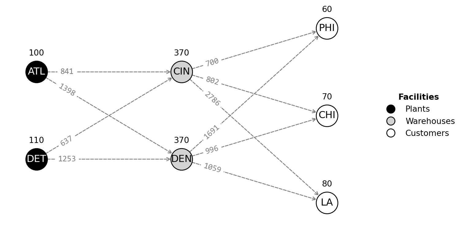
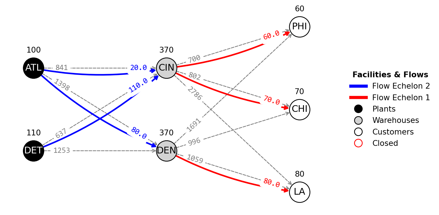
Figure 10.1 shows the transportation network.

Formulate this scenario as an optimization model with the primary objective of minimizing distribution costs.

Figure 10.1: The transportation costs (edges) and facility capacities and customer demands (over the nodes).

Answer

Set parameter Username
Set parameter LicenseID to value 2777413
Academic license - for non-commercial use only - expires 2027-02-10

This is a network problem with decision variables $x_{ij}$, where $(i, j)$ denotes an arc in the network that represents the quantity of goods shipped from node $i$ to node $j$.

The objective is to minimize the total distribution cost, which is modeled as follows:

\[ \begin{align} \min \, \, & 10000(x_{DET,DEN} + x_{DET,CIN} + x_{ATL,DEN} + x_{ATL,CIN}) \\ &+ 1253x_{DET,DEN} + 637x_{DET,CIN} \\ &+ 1398x_{ATL,DEN} + 841x_{ATL,CIN} \\ &+ 1059x_{DEN,LA} + 996x_{DEN,CHI} + 1691x_{DEN,PHI} \\ &+ 2786x_{CIN,LA} + 802x_{CIN,CHI} + 700x_{CIN,PHI} \\ \end{align} \]

subject to the following constraints:

Plant capacity constraints ensure that the number of goods shipped from Detroit and Atlanta does not exceed their production capacities.

\[ \begin{align} x_{DET,DEN} + x_{DET,CIN} \leq 110 \\ x_{ATL,DEN} + x_{ATL,CIN} \leq 100 \end{align} \]
Conservation of flow constraints require that the number of goods shipped out of Denver and Cincinnati equals the number of goods received by the plants, ensuring that all goods are accounted for and there’s no accumulation at the warehouses.

\[ \begin{align} x_{DET,DEN} + x_{ATL,DEN} = x_{DEN,LA} + x_{DEN,CHI} + x_{DEN,PHI} \\ x_{DET,CIN} + x_{ATL,CIN} = x_{CIN,LA} + x_{CIN,CHI} + x_{CIN,PHI} \end{align} \]
Demand constraints guarantee that the goods shipped to Los Angeles, Chicago, and Philadelphia meet the minimum weekly requirements.

\[ \begin{align} x_{DEN,LA} + x_{CIN,LA} \geq 80 \\ x_{DEN,CHI} + x_{CIN,CHI} \geq 70 \\ x_{DEN,PHI} + x_{CIN,PHI} \geq 60 \\ \end{align} \]
The weekly capacity of the warehouses is not exceeded.

\[ \begin{align*} & x_{DET,DEN} + x_{ATL,DEN} + x_{SA,DEN} \leq 370 \\ & x_{DET,CIN} + x_{ATL,CIN} + x_{SA,CIN} \leq 370 \end{align*} \]

Non-negativity constraints ensure that the decision variables cannot take on negative values.

\[ \forall (i,j),\ x_{ij} \geq 0 \]

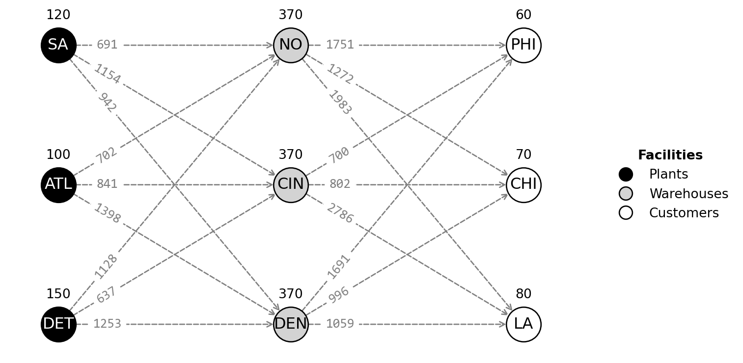
Figure 10.2: The minimum distribution cost is 2,481,590.0.

Exercise 10.2 (Automotive Company Capacitated Facility Location Problem) Metal Motors is an automotive company that must optimize its distribution system to minimize costs. The company’s operations include production at plants, storage at warehouses, and delivery to customers. The current infrastructure comprises:

Plants: Detroit (DET), Atlanta (ATL), and a newly opened plant in San Antonio (SA)
Warehouses: Denver (DEN), Cincinnati (CIN), and a new warehouse in New Orleans (NO)
Customers: Located in Los Angeles (LA), Chicago (CHI), and Philadelphia (PHI)

The production capacity per week is as follows:

Detroit (DET): 150 cars
Atlanta (ATL): 100 cars
San Antonio (SA): 120 cars

The customer demand per week is as follows:

Los Angeles (LA): 80 cars
Chicago (CHI): 70 cars
Philadelphia (PHI): 60 cars

Each warehouse can store at most 370 cars per week.

The production cost for each car at any plant is $10,000. Table 10.3 shows the shipping costs from cars from plants to warehouses, and Table 10.4 shows the shipping costs from warehouses to customers.

Table 10.3: Costs of shipping a car from plants to warehouses

From/To	Denver (DEN)	Cincinnati (CIN)	New Orleans (NO)
Detroit (DET)	$1253	$637	$1128
Atlanta (ATL)	$1398	$841	$702
San Antonio (SA)	$942	$1154	$691

Table 10.4: Costs of shipping a car from warehouses to customers

From/To	Los Angeles (LA)	Chicago (CHI)	Philadelphia (PHI)
Denver (DEN)	$1059	$996	$1691
Cincinnati (DEN)	$2786	$802	$700
New Orleans (NO)	$1983	$1272	$1751

Setup costs for each facility are as follows:

	Detroit (DET)	Atlanta (ATL)	San Antonio (SA)	Denver (DEN)	Cincinnati (CIN)	New Orleans (NO)
Setup cost	$20,000	$18,000	$10,000	$5,000	$6,000	$50,000

Management is faced with strategic decisions regarding which plants and warehouses to operate to satisfy customer demand at the lowest possible cost. These decisions include:

Determining the number of cars to produce and ship from each plant to each warehouse.
Deciding the number of cars to distribute from each warehouse to each customer.
Selecting which plants and warehouses should be operational, considering the setup costs.

Formulate an optimization model that minimizes the total cost of production, shipping, and facility setup while meeting or exceeding customer demand and not exceeding plant production capacities and warehouse capacities.

Figure 10.3: The transportation network.

Answer

Automotive Company Capacitated Facility Location Problem (Solution). First, add a new variable related to opening a new depot:

\[ y_i = \begin{cases} 1, & \text{if plant/warehouse i is open,} \\ 0, & \text{otherwise,} \end{cases} \]

The model aims to minimize the total cost, which includes production, shipping, and setup costs for plants and warehouses. The objective function is:

\[ \begin{align*} \min \quad & 10000(x_{DET,DEN} + x_{DET,CIN} + x_{DET,NO} + x_{ATL,DEN} + x_{ATL,CIN}) \\ & + 10000(x_{ATL,NO} + x_{SA,DEN} + x_{SA,CIN} + x_{SA,NO}) \\ & + 1253x_{DET,DEN} + 637x_{DET,CIN} + \ldots + 1983x_{NO,LA} \\ & + 1272x_{NO,CHI} + 1751x_{NO,PHI} \\ & + 20000y_{DET} + 18000y_{ATL} + 10000y_{SA} \\ & + 5000y_{DEN} + 6000y_{CIN} + 5000y_{NO} \end{align*} \]

subject to the following constraints:

The production capacity constraints ensure that the quantity of cars shipped from each plant does not exceed its capacity, which is a function of whether the plant is open or not.

\[ \begin{align*} & x_{DET,DEN} + x_{DET,CIN} + x_{DET,NO} \leq 150y_{DET} \\ & x_{ATL,DEN} + x_{ATL,CIN} + x_{ATL,NO} \leq 100y_{ATL} \\ & x_{SA,DEN} + x_{SA,CIN} + x_{SA,NO} \leq 120y_{SA} \end{align*} \]
The flow conservation constraints require that the cars shipped from the plants to the warehouses match the cars shipped from warehouses to the customers, ensuring a balanced flow.

\[ \begin{align*} & x_{DET,DEN} + x_{ATL,DEN} + x_{SA,DEN} = x_{DEN,LA} + x_{DEN,CHI} + x_{DEN,PHI} \\ & x_{DET,CIN} + x_{ATL,CIN} + x_{SA,CIN} = x_{CIN,LA} + x_{CIN,CHI} + x_{CIN,PHI} \\ & x_{DET,NO} + x_{ATL,NO} + x_{SA,NO} = x_{NO,LA} + x_{NO,CHI} + x_{NO,PHI} \end{align*} \]
Each customer’s demand is met or exceeded.

\[ \begin{align*} & x_{DEN,LA} + x_{CIN,LA} + x_{NO,LA} \geq 80 \\ & x_{DEN,CHI} + x_{CIN,CHI} + x_{NO,CHI} \geq 70 \\ & x_{DEN,PHI} + x_{CIN,PHI} + x_{NO,PHI} \geq 60 \end{align*} \]
The weekly capacity of the warehouses is not exceeded.

\[ \begin{align*} & x_{DET,DEN} + x_{ATL,DEN} + x_{SA,DEN} \leq 370y_{DEN} \\ & x_{DET,NO} + x_{ATL,NO} + x_{SA,NO} \leq 370y_{NO} \\ & x_{DET,CIN} + x_{ATL,CIN} + x_{SA,CIN} \leq 370y_{CIN} \end{align*} \]

Non-negativity constraints ensure the shipped quantities cannot be negative.

\[ x_{ij} \geq 0 \]
The binary constraints indicate whether a plant or warehouse is open (1) or closed (0).

\[ y_{i} \in \{0,1\} \]

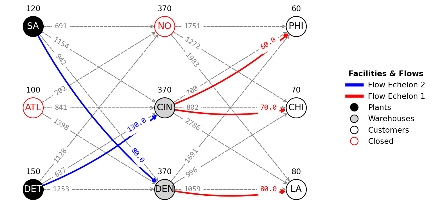
Figure 10.4 shows the connection between the different locations and the flow between the opened facilities.

Figure 10.4: The minimum distribution cost is 2,482,030.0 and the closed facilities are ATL, NO.

Exercise 10.3 (Optimization of a Joint-Use Multiproduct Oil Pipeline Network) Two oil-producing companies are collaborating on the design of a multiproduct oil pipeline network for shared use. This network will facilitate regular oil transportation between specific pairs of origin and destination nodes.

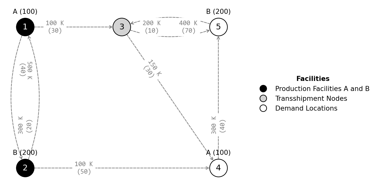
The first company operates a production facility at node 1, with a daily output of 100 units destined for node 4. The second company’s production occurs at node 2, from where 200 units are transported daily to node 5. The two types of oil products differ and are assigned a uniform shipping cost of 50 per unit. The potential pipeline routes are depicted by the arcs in the network diagram shown in Figure 10.5, and the capacity of each pipeline is quantified as multiples of a standard unit of capacity. The fixed construction costs associated with each pipeline capacity are detailed in Table 10.5.

For instance, constructing a pipeline between nodes 1 and 3 allows for a capacity of 30 tonnes, incurring a fixed cost of 500,000. Installing two such pipelines doubles the capacity to 60 tonnes, with the cost rising linearly to 1,000,000.

Table 10.5: Installation costs and capacities of pipelines.

Pipeline	Fixed cost per unit of pipeline installed	Pipeline Capacity (tonnes)
(1,2)	500,000	40
(2,1)	300,000	20
(1,3)	100,000	30
(2,4)	100,000	50
(3,4)	150,000	30
(3,5)	200,000	10
(4,5)	300,000	40
(5,3)	400,000	70

Figure 10.5: Network design. Edge labels in the network diagram are formatted as $c_{ij}(u_{ij})$, where $c_{ij}$ represents the fixed cost per unit of pipeline installed and $u_{ij}$ represents the capacity between nodes $i$ and $j$. Commodity A requires a delivery of 100 units from node 1 to node 4, while commodity B demands the transportation of 200 units from node 2 to node 5.

Answer

This optimization scenario addresses a specific case within the Multicommodity Capacitated Fixed-Charge Network Design Problem (MCND) (see an example of a typical formulation by Gendron, Hanafi, and Todosijevic (2016)). It is modeled on a directed graph $G = (N, A)$, with $N$ representing the nodes and $A$ representing the arcs.

In this context, we have:

Sets and Indices:
- $N$: Set of nodes in the network.
- $A$: Set of arcs representing potential pipelines.
- $K$: Set of commodities to be routed through the network.
Parameters:
- $c_{ij}$: Transportation cost per unit on arc $(i, j)$.
- $f_{ij}$: Fixed design cost for using arc $(i, j)$.
- $d_k$: Demand for commodity $k$.
- $u_{ij}$: Capacity of arc $(i, j)$.
- $N_i^+$: Set of outgoing nodes from node $i$.
- $N_i^-$: Set of incoming nodes to node $i$.
- $O_k$: Origin node for commodity $k$.
- $D_k$: Destination node for commodity $k$.
Variables:
- $x_{ij}^k$: Flow of commodity $k$ on arc $(i, j)$.
- $y_{ij}$: Integer variable indicating the number of units of pipeline installed on arc $(i, j)$.

The objective is to minimize the total cost composed of the transportation cost across all commodities and arcs, as well as the fixed cost associated with constructing pipelines:

\[ \min z = \sum_{k \in K} \sum_{(i,j) \in A} c_{ij} x_{ij}^k + \sum_{(i,j) \in A} f_{ij} y_{ij} \]

The following constraints are applied:

Flow conservation for each commodity at each node: \[ \sum_{j \in N_i^+} x_{ij}^k - \sum_{j \in N_i^-} x_{ji}^k = \begin{cases} d_k & \text{if } i = O_k, \\ -d_k & \text{if } i = D_k, \\ 0 & \text{otherwise} \end{cases} \quad \forall i \in N, \forall k \in K \]
Capacity limits for each pipeline: \[ \sum_{k \in K} x_{ij}^k \leq u_{ij} y_{ij} \quad \forall (i, j) \in A \]
Non-negativity of flow variables: \[ x_{ij}^k \geq 0 \quad \forall (i, j) \in A, \forall k \in K \]
Integrality of pipeline unit variables: \[ y_{ij} \in \mathbb{Z} \quad \forall (i, j) \in A \]

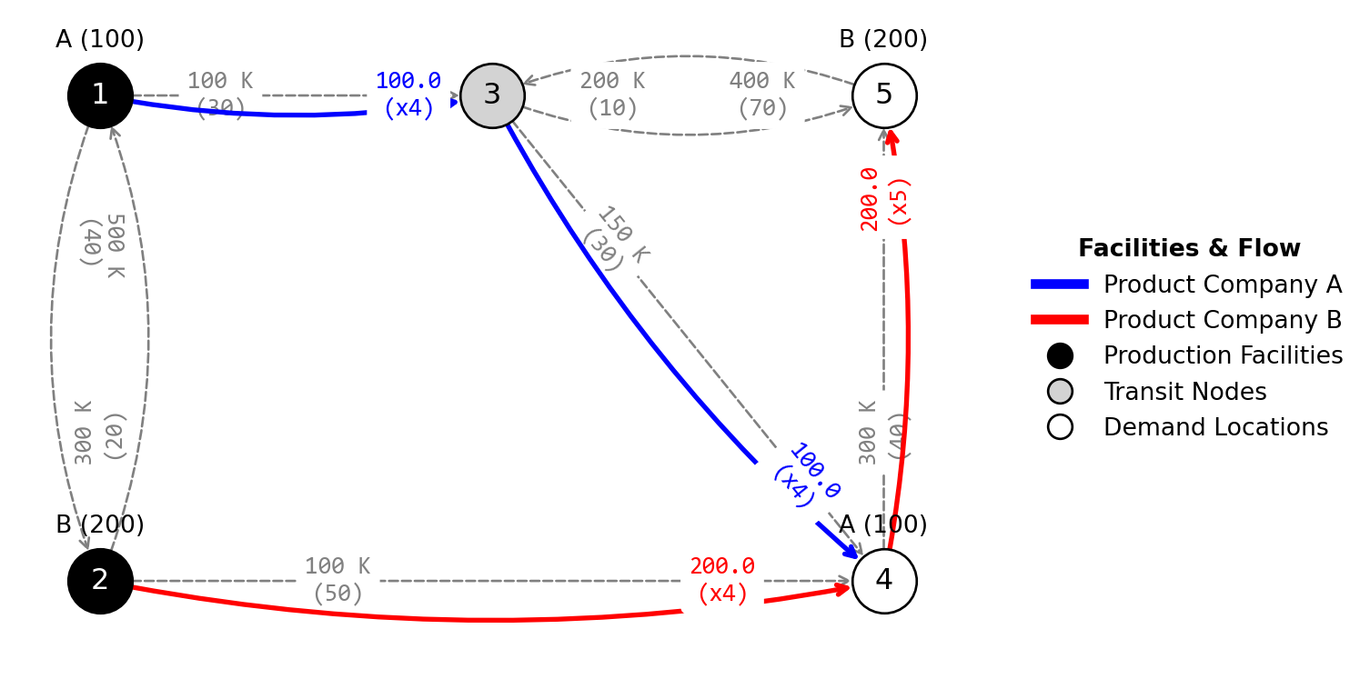
Figure 10.6 shows the solution of this scenario. In Summary:

Build 4 pipelines connecting nodes 1 and 3
Build 4 pipelines connecting nodes 2 and 4
Build 4 pipelines connecting nodes 3 and 4
Build 5 pipelines connecting nodes 4 and 5
Transport 100 tonnes of product A from node 1 to node 3
Transport 200 tonnes of product B from node 2 to node 4
Transport 100 tonnes of product A from node 3 to node 4
Transport 200 tonnes of product B from node 4 to node 5

The total cost of deploying this network design is 2,930,000.00.

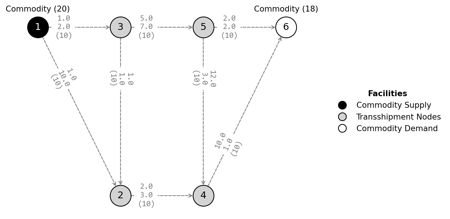
Figure 10.6: Optimized network design. Edge labels are formatted as $c_{ij}(u_{ij})$, where $c_{ij}$ is the cost per unit of pipeline installed and $u_{ij}$ is the capacity of a pipeline connection between nodes $i$ and $j$. The commodity A has a demand of 100 that must be routed from node 1 to 4, and the commodity B has a demand of 200 that must be routed from node 2 to 5. Colored edge labels are formatted as $x_{ij}(y_{ij})$, where $x_{ij}$ is the flow between nodes $i$ and $j$, and $y_{ij}$ is the number of pipelines installed between $i$ and $j$.

Exercise 10.4 (Multi-Objective Transportation Network Design Problem) Given the network depicted in Figure 10.7 where each arc is labeled with values $c_{ij}, t_{ij}, u_{ij}$, representing the cost per unit $c_{ij}$ and the travel time $t_{ij}$ for transportation between nodes $i$ and $j$ with capacity $u_{ij}$, the goal is to formulate an optimization problem. Node 1 acts as the supplier providing 20 units of a commodity, and node 6 is the demand point requiring 18 units. It is required to route these units through the network while minimizing the total cost and time, subject to the following conditions:

All arcs have a capacity restriction of 10 units.
The supply at node 1 is 20 units.
The demand at node 6 is 18 units.
The network aims to minimize the total cost and time.

Figure 10.7: Network design. Edge labels in the network diagram are formatted as $c_{ij} t_{ij} (u_{ij})$, where $c_{ij}$ represents the cost, $t_{ij}$ represents the time and $u_{ij}$ represents the capacity between nodes $i$ and $j$.

Answer

This is a transportation network design problem similar to those encountered in previous exercises. However, in this case, we observe that costs and time are measured in different units, and no direct transformation between the two is provided. Therefore, a multi-objective optimization approach is necessary. Available methods include the epsilon-constraint method, goal programming, lexicographic, and weighted sum method. Since no specific goals are stated, goal programming is not applicable. Similarly, without weights for the objectives (cost and time), the weighted sum method is also less suitable. This leaves us with the epsilon-constraint and lexicographic methods as the most viable options.

In the absence of priorities between objectives, we could first minimize the cost and then the time, or vice versa. Using the epsilon-constraint method, we would introduce a new constraint where the sum of all arcs is constrained by a specified epsilon. Epsilon could be heuristically determined by considering that at least two paths must be utilized from node 1 to node 6, due to the capacity restriction on the arcs.

With the lexicographic method, we prioritize one objective over the other. The first objective (either cost or time) is minimized, and its optimal value is then used as a constraint when minimizing the second objective. This process ensures that the solution optimizes the primary objective without compromising the optimal value already obtained.

Considering minimizing cost has higher priority than time, we have the following formulation:

Sets and Indices:

$N$: Set of nodes in the network, where $N = \{1, 2, 3, 4, 5, 6\}$.
$A$: Set of arcs representing potential pathways in the network.

Parameters:

$c_{ij}$: Cost per unit for transporting commodities through arc $(i, j)$.
$t_{ij}$: Travel time per unit for arc $(i, j)$.
$u_{ij}$: Capacity of arc $(i, j)$, where $u_{ij} = 10$ for all arcs.
$s$: Supply at the supplier node (node 1), where $s = 20$ units.
$d$: Demand at the demand node (node 6), where $d = 18$ units.

Decision Variables:

$x_{ij}$: Number of units transported through arc $(i, j)$.

Constraints:

Supply constraint at node 1: \[ \sum_{j:(1,j) \in A} x_{1j} = s \]

Demand constraint at node 6: \[ \sum_{i:(i,6) \in A} x_{i6} = d \]

Capacity constraints on each arc: \[ x_{ij} \leq u_{ij} \quad \forall (i, j) \in A \]

Flow conservation constraints at transshipment nodes: \[ \sum_{j:(i,j) \in A} x_{ij} - \sum_{j:(j,i) \in A} x_{ji} = 0 \quad \forall i \in N \setminus \{1, 6\} \]

Non-negativity and integrality of flow variables: \[ x_{ij} \geq 0 \quad \forall (i, j) \in A \]

\[ x_{ij} \in \mathbb{Z}^{+} \quad \forall (i, j) \in A \]

Lexicographic optimization approach. Since we consider minimizing cost and time, we have to solve a sequence of optimization problems. We prioritize one objective first and, once solved, use its solution as a constraint when optimizing the second objective.

First Stage: Minimize Costs

Objective Function: \[ \min Z_1 = \sum_{(i,j) \in A} c_{ij} x_{ij} \]

Subject to the same constraints as in the previous formulation.

Second Stage: Minimize Time with Cost Constraint

Objective Function: \[ \min Z_2 = \sum_{(i,j) \in A} t_{ij} x_{ij} \]

Subject to the constraints previously formulated plus an additional constraint that the cost does not exceed the optimal cost found in the first stage:

\[ \sum_{(i,j) \in A} c_{ij} x_{ij} \leq Z_1^* \]

Here $Z_1^*$ represents the optimal total cost found in the first stage. The second stage optimization is only performed on feasible solutions that achieve this cost.

Exercise 10.5 (LTL Freight Rates and Weight Brackets) LTL tariffs create a piecewise-linear freight cost curve. The key idea is that a higher weight bracket can sometimes produce a lower total freight charge, so it may be worth adding a small amount of freight to reach the next bracket.

Units

The carrier tariff is published in pounds and CWT, so the original carrier units are retained here. One CWT equals 100 lb.

Table 10.6: Nominal LTL freight rates by weight bracket.

	Min Weight (lb)	Max Weight (lb)	Rate ($/CWT)	Rate ($/lb)
1	1	499	107.75	1.0775
2	500	999	92.26	0.9226
3	1000	1999	71.14	0.7114
4	2000	4999	64.14	0.6414
5	5000	9999	52.21	0.5221
6	10000	19999	40.11	0.4011
7	20000	29999	27.48	0.2748

Using Table 10.6, do the following:

Identify the nominal weight breakpoints and freight rates.
Determine the upgrade thresholds: the shipment weights at which it becomes cheaper to add more freight and qualify for the next bracket.
Suppose there are $N$ candidate products. Product $i$ has weight $w_i$, and at least $W^{\text{req}}$ pounds must be shipped. Use a lambda formulation of the freight cost function to decide which products to include so that total freight cost is minimized.
Solve the illustrative instance with product weights $[100, 200, 300, 400, 500, 600, 700, 800, 900, 1000]$ lb and $W^{\text{req}} = 4300$ lb using Gurobi.

Answer

The nominal breakpoints are the lower limits of the carrier table: $1$, $500$, $1000$, $2000$, $5000$, $10000$, and $20000$ lb.

The corresponding nominal freight rates are: $107.75$, $92.26$, $71.14$, $64.14$, $52.21$, $40.11$, and $27.48$ dollars per CWT.

Upgrade Thresholds

Let $L_k$ be the minimum weight of bracket $k$ and let $r_k$ be its rate in dollars per pound. If a shipment currently sits in bracket $k$, it becomes attractive to move to bracket $k + 1$ when the current freight charge equals the minimum charge of the next bracket:

\[ r_k x = r_{k + 1} L_{k + 1}. \]

Therefore, the upgrade threshold between brackets $k$ and $k + 1$ is

\[ \bar{x}_k = \left\lceil \frac{r_{k + 1} L_{k + 1}}{r_k} \right\rceil. \]

Table 10.7: Upgrade thresholds between consecutive weight brackets.

	Current Bracket	Upgrade Threshold (lb)	Ship at Least (lb)	New Total Charge ($)
1	1--499 lb	429	500	461.3
2	500--999 lb	772	1000	711.4
3	1000--1999 lb	1804	2000	1282.8
4	2000--4999 lb	4071	5000	2610.5
5	5000--9999 lb	7683	10000	4011.0
6	10000--19999 lb	13703	20000	5496.0

Table 10.7 gives the practical trigger points:

From $429$ to $499$ lb, it is cheaper to move to $500$ lb.
From $772$ to $999$ lb, it is cheaper to move to $1000$ lb.
From $1804$ to $1999$ lb, it is cheaper to move to $2000$ lb.
From $4071$ to $4999$ lb, it is cheaper to move to $5000$ lb.
From $7683$ to $9999$ lb, it is cheaper to move to $10000$ lb.
From $13703$ to $19999$ lb, it is cheaper to move to $20000$ lb.

Table 10.8: Segment endpoint data for the lambda formulation.

	Min Weight (lb)	Max Weight (lb)	Rate ($/CWT)	Rate ($/lb)	Lower Cost ($)	Upper Cost ($)
1	1	499	107.75	1.0775	1.0775	537.6725
2	500	999	92.26	0.9226	461.3000	921.6774
3	1000	1999	71.14	0.7114	711.4000	1422.0886
4	2000	4999	64.14	0.6414	1282.8000	3206.3586
5	5000	9999	52.21	0.5221	2610.5000	5220.4779
6	10000	19999	40.11	0.4011	4011.0000	8021.5989
7	20000	29999	27.48	0.2748	5496.0000	8243.7252

Modeling point

The rounded upgrade thresholds explain the freight discount logic, but the optimization model itself should use the nominal tariff segments. That is because the selected shipment weight is a decision variable, not a fixed input.

Lambda Formulation

Let $I = \{1, \ldots, N\}$ be the set of candidate products and let $K$ be the set of weight brackets.

Parameters:

$w_i$: weight of product $i$.
$L_k$: lower bound of bracket $k$.
$U_k$: upper bound of bracket $k$.
$r_k$: freight rate of bracket $k$ in dollars per pound.
$C_k^{L} = r_k L_k$: freight cost at the lower endpoint of bracket $k$.
$C_k^{U} = r_k U_k$: freight cost at the upper endpoint of bracket $k$.
$W^{\text{req}}$: minimum total weight that must be shipped.

Decision variables:

$y_i \in \{0, 1\}$: equals $1$ if product $i$ is shipped.
$z_k \in \{0, 1\}$: equals $1$ if bracket $k$ is selected.
$\lambda_{k,1} \ge 0$: lambda weight on the lower endpoint of bracket $k$.
$\lambda_{k,2} \ge 0$: lambda weight on the upper endpoint of bracket $k$.
$x \ge 0$: total shipped weight.
$TC \ge 0$: total freight cost.

Objective:

\[ \min TC \]

Subject to:

\[ x = \sum_{i \in I} w_i y_i \]

\[ x \ge W^{\text{req}} \]

\[ \sum_{k \in K} z_k = 1 \]

\[ \sum_{k \in K} (L_k \lambda_{k,1} + U_k \lambda_{k,2}) = x \]

\[ \sum_{k \in K} (C_k^{L} \lambda_{k,1} + C_k^{U} \lambda_{k,2}) = TC \]

\[ \lambda_{k,1} + \lambda_{k,2} = z_k \quad \forall k \in K \]

\[ y_i \in \{0, 1\} \quad \forall i \in I \]

\[ z_k \in \{0, 1\} \quad \forall k \in K \]

\[ \lambda_{k,1}, \lambda_{k,2} \ge 0 \quad \forall k \in K \]

This formulation uses two lambda variables for each bracket. If bracket $k$ is active, then $z_k = 1$ and the pair $(\lambda_{k,1}, \lambda_{k,2})$ interpolates between the lower and upper endpoints of that bracket. All lambda variables in inactive brackets are forced to zero.

The number of products shipped is

\[ \sum_{i \in I} y_i. \]

If all products must be shipped, replace the selection decision with $y_i = 1$ for all $i \in I$.

Optimal Gurobi Solution

Table 10.9: Optimal solution of the illustrative lambda-model instance.

	Metric	Value
0	Required Weight (lb)	4300
1	Optimal Weight (lb)	5000.0
2	Freight Cost ($)	2610.5
3	Active Bracket	5
4	Products Shipped	8
5	Selected Weights (lb)	200, 300, 500, 600, 700, 800, 900, 1000

For this illustrative instance, Gurobi chooses an optimal shipment of 5,000 lb in bracket 5, with total freight cost $2,610.50.

10.1 Exercises

10.2 References