14 Facility-location optimization

There are three things that matter in property: location, location, location. Lord Harold Samuel

Learning objectives

distinguish facility-location problem types;
compare single- and multi-warehouse networks;
classify models by level, allocation, hierarchy, and flow; and
select an exact, heuristic, simulation, or multi-criteria method.

Facility-location problems

Facility-location problems select sites to minimize cost or maximize service. The main variants include:

Core cost–distance models
Multi-echelon and hierarchical models
Coverage-based models
Median and center models

Core cost–distance models

Used for single-level facility siting.

FLP (Facility Location Problem): Choose facility sites to minimize cost or maximize service, given a cost or distance structure.
FLAP (Facility Location and Allocation Problem): Jointly choose facility sites and customer assignments. Differs from FLP by including assignment decisions (e.g., each customer must be assigned to exactly one facility).
WLP (Warehouse Location Problem): FLP specialized to warehousing and distribution, often with capacity or service constraints.

Multi-echelon and hierarchical models

Used for multi-level supply chains.

DCLP (Distribution Center Location Problem): Two-level siting with flows from plants to DCs to customers.
MLFLP (Multi-Level Facility Location Problem): Predefined levels and tiered flow constraints between levels (e.g., always plant → regional hub → DC → customer).
HFLP (Hierarchical Facility Location Problem): Multiple facility types across levels with level-specific service rules but with flexibility for bypassing levels (e.g., plant → regional hub → DC → customer, or plant → regional hub → customer).

Coverage-based models

Used to ensure service coverage within a specified threshold.

LSCP (Location Set Covering Problem): Minimize the number of facilities so all demand is covered within a service threshold (e.g., distance or time).
MCLP (Maximal Covering Location Problem): Given a budget of at most \(p\) sites, maximize covered demand (within a service threshold).

Median and center models

Used to optimize service distances.

p-Median: Open exactly \(p\) facilities to minimize total demand-weighted distance (i.e., average distance).
p-Center: Open exactly \(p\) facilities to minimize the maximum distance to any customer (i.e., worst-case service).

Taxonomy of facility-location problems

Table 14.1 compares variants across:

Facility levels (single, two, multi)
Customer allocation (optional, yes, no)
Hierarchy (no = flat, yes = multi-level)
Flow (direct = one step, tiered = fixed multistage, flexible = bypasses allowed)
Typical applications

Table 14.1: Allocation and hierarchy distinguish the main facility-location models.

Type	Facility levels	Allocation	Hierarchy	Flow	Typical Application
FLP	Single	Optional	No	Direct	General facility placement
FLAP	Single	Yes	No	Direct	Joint siting and assignment
WLP	Single or Two	Yes	Usually no	Direct	Warehousing and distribution
DCLP	Two	Yes	Yes (Plant-DC-Customer)	Tiered	Multi-echelon supply chains
HFLP	Multi	Yes	Yes (optimization-based)	Tiered or Flexible	Health care, telecom, complex logistics
MLFLP	Multi	Yes	Yes (predefined)	Tiered	Structured supply chains
LSCP	Single	No (cover)	No	Direct	Emergency services, coverage planning
MCLP	Single	No (cover)	No	Direct	Retail, public service siting
p-Median	Single	Yes	No	Direct	Cost-distance minimization
p-Center	Single	Yes	No	Direct	Minimax service radius

Single- and multi-warehouse trade-offs

Trade-offs depend on demand geography, service targets, and scale economies.
Factor	Single Warehouse	Multi-Warehouse
Fixed Costs	Lower	Higher
Transport Costs	Often higher	Often lower
Inventory Costs	Lower through risk pooling	Higher due to fragmentation
Customer Service	Slower average delivery	Faster average delivery
Supply Chain Risk	Concentration risk	Redundancy and geographical diversification
Capacity growth	Limited by single-site capacity	Capacity can expand by region
Sustainability	More transport emissions on average	Larger facility footprint, transport can improve

Classifications of facility-location problems

Single- or multi-facility: One facility or several facilities.
Static or dynamic: Fixed parameters or parameters that change by planning stage.
Single- or multi-period: One time period or several time periods.
Deterministic or stochastic: Known or uncertain parameters.
Single- or multi-echelon: Direct customer supply or several distribution layers.
Capacitated or uncapacitated: Limited or unlimited facility capacity.
Single- or multi-flow: Fixed or flexible paths through the hierarchy.
Single- or multi-objective: One criterion or several criteria.

Optimization techniques

Exact methods: branch and bound, branch and cut, Lagrangian relaxation, Benders decomposition, and column generation.
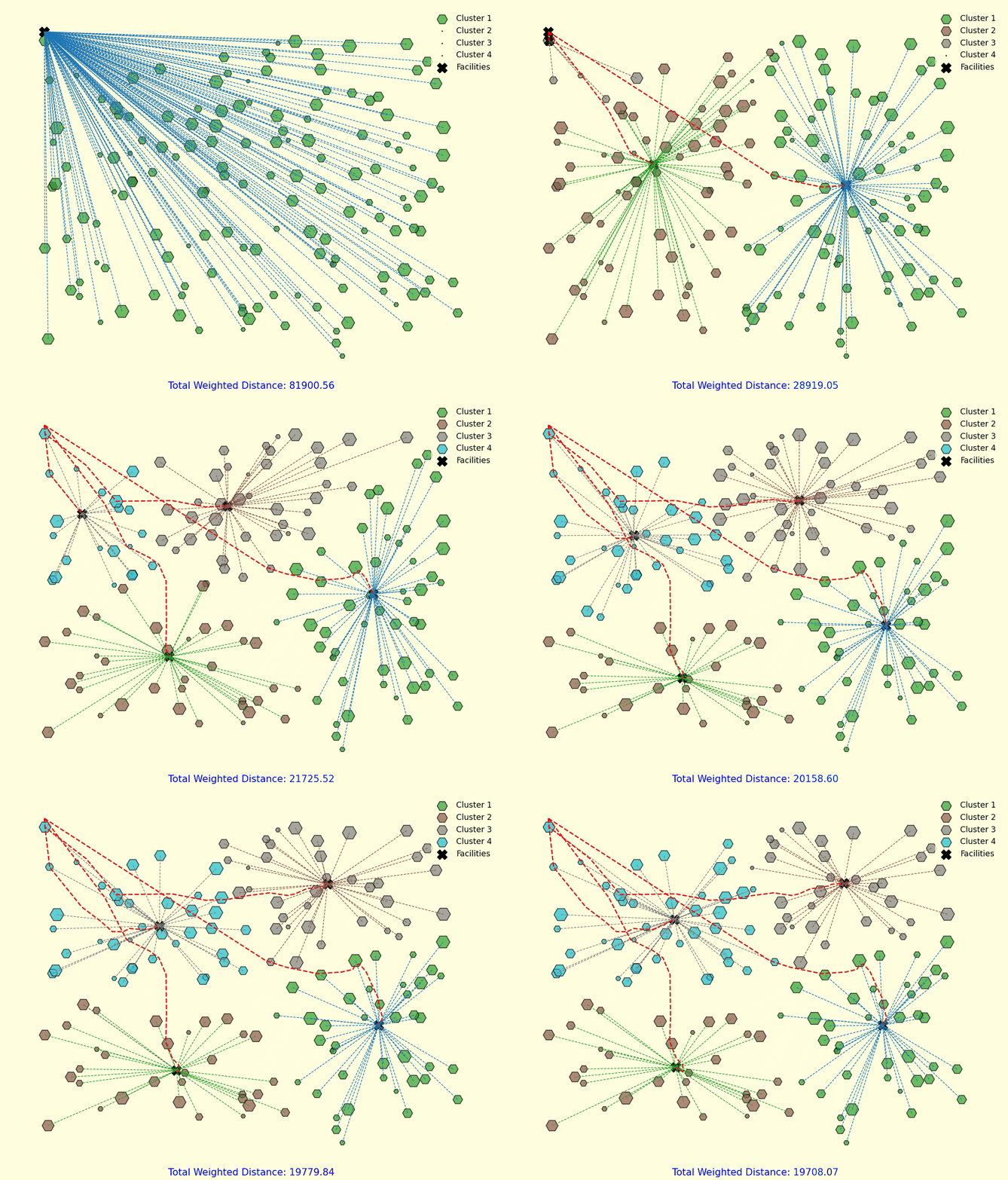
Heuristic methods: center of gravity, k-means-style clustering, greedy construction, local search, and interchange.
Metaheuristics: genetic algorithms, simulated annealing, tabu search, variable-neighborhood search, particle swarm, and ant colony.
Other approaches: discrete-event simulation, machine-learning-assisted design, and multi-criteria decision-making.

Exact method: p-median

Goal: Select \(p\) facilities to minimize total distance between customers and assigned facilities.

\[ \min \sum_{i \in I}\sum_{j \in J} d_{ij} x_{ij} \]

Subject to

\(x_{ij} \le y_j \quad \forall i \in I,\ j \in J\) (assign only to open facilities)
\(\sum_{j \in J} y_j = p\) (exactly \(p\) facilities opened)
\(x_{ij},\ y_j \in \{0,1\}\) (binary variables)

where:

\(I\): set of customers
\(J\): set of potential facility locations
\(d_{ij}\): distance from customer \(i\) to facility \(j\)
\(x_{ij}\): binary variable, 1 if customer \(i\) assigned to facility \(j\), 0 otherwise
\(y_j\): binary variable, 1 if facility \(j\) is opened, 0 otherwise
\(p\): number of facilities to open

Exact method: warehouse location problem (WLP)

Goal: Decide whether to open facilities and assign customers to minimize total fixed and variable costs.

\[ \min \sum_{j \in J} f_j y_j + \sum_{i \in I} \sum_{j \in J} c_{ij} x_{ij} \]

Subject to

\(\sum_{j \in J} x_{ij} = 1 \quad \forall i \in I\) (each customer assigned to one facility)
\(x_{ij} \le y_j \quad \forall i \in I,\ j \in J\) (assign only to open facilities)
\(x_{ij} \in \{0,1\},\ y_j \in \{0,1\}\) (binary variables)

where:

\(I\): set of customers
\(J\): set of potential facility locations
\(f_j\): fixed cost to open facility \(j\)
\(c_{ij}\): cost to serve customer \(i\) from facility \(j\)
\(x_{ij}\): binary variable, 1 if customer \(i\) assigned to facility \(j\), 0 otherwise
\(y_j\): binary variable, 1 if facility \(j\) is opened, 0 otherwise

Heuristic methods

Heuristics generate solutions without an optimality guarantee. They can handle large instances or constraints that make exact models slow.

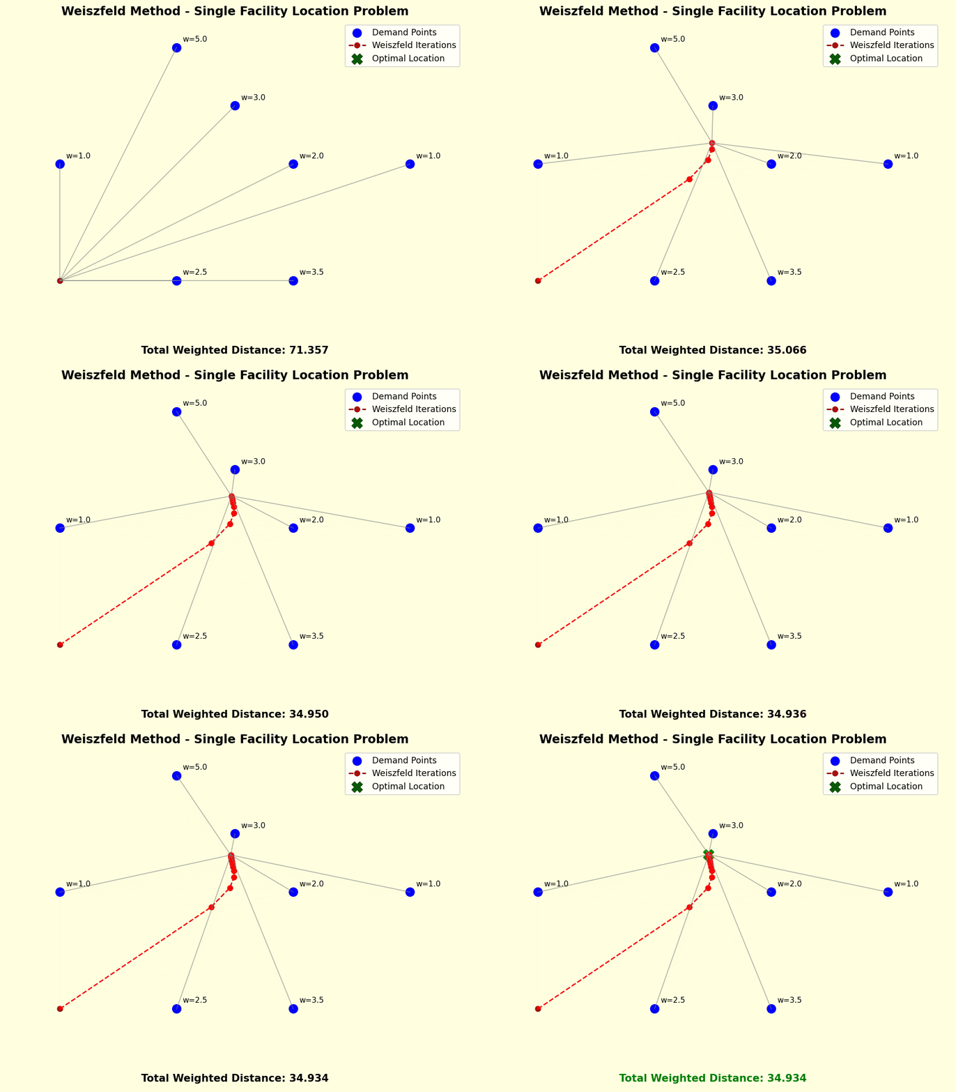
Example: Weiszfeld’s algorithm

Weiszfeld’s algorithm is an iterative technique for solving the single-facility location problem in Euclidean space.
It determines the optimal location that minimizes the weighted total distance to a set of demand points.
Weights represent the importance of each demand point in the optimization process.

(a) Single facility location (optimal within error bounds)

Metaheuristic methods

Example GA workflow for WLP:

Initialization: Generate an initial population of warehouse-location solutions.
Selection: Evaluate solutions and select parents.
Crossover: Combine pairs of parents to create offspring.
Mutation: Introduce random changes in offspring.
Replacement: Replace lower-fitness solutions with offspring.
Termination: Stop at the iteration limit or convergence criterion.

Discrete-event simulation (DES)

Model order arrivals, processing, dispatch, and travel.
Compare candidate location sets on delivery time, service level, and resource use.
Use simulation outputs to validate and tune optimization results.

Machine learning (ML)

Demand forecasting with time series or ML models.
Customer clustering for service regions or capacity planning.

Multi-criteria decision-making (MCDM)

AHP or BWM to prioritize location candidates.
Pareto analysis to identify non-dominated solutions for cost, service, and emissions.

Single-objective optimization

Cost minimization: fixed facility, transport, handling, inventory.
Sustainability: estimated emissions from transport and operations.
Service level: delivery time, fill rate, distance constraints.

Multi-objective optimization

Weighted Sum: scalarize with stakeholder weights.
\(\varepsilon\)-Constraint: optimize one objective subject to bounds on others.
Pareto-Based Evolutionary Algorithms: for example, NSGA-II to approximate the frontier.

Exercises

Urban Distribution Network Design. A fast e-grocery company expands in Enschede. Target 10-minute deliveries. Decide how many urban warehouses to open and where, balancing cost, service level, and operational feasibility.

Define how to represent customers (e.g., geocoded demand points, aggregated zones, or a grid)
Define the number of customers (e.g., investigate scenarios with 100, 500, 1000 customers, use actual demand, etc.)
Choose a distance metric (e.g., Euclidean, Manhattan, or network distance via road network)
Define candidate warehouse locations (e.g., existing buildings, commercial zones, or a grid)
Create distance matrix between customers and candidate locations
Decide how you will convert distances to travel times (e.g., average speed assumptions, traffic data)
Apply an optimization method (e.g., exact, heuristic, metaheuristic) to select warehouse locations and assign customers