| Quantity | Value |
|---|---|
| Distance (m) | 12.0 |
| Travel time (s) | 10.0 |
| Picking time (s) | 6.0 |
| Tour duration (s) | 16.0 |
| Items collected | 2.0 |
| Completed orders | 2.0 |
Order picking: routing, batching, and scheduling
Aim
Compare picking routes, order batches, and picker assignments for a fixed order workload. Use the results to explain changes in walking distance and completion time.
Learning objectives
After completing this tutorial, you will be able to:
- generate and check tours that collect every assigned item and return to the depot;
- compare routing and batching methods on the same orders;
- assign tours to pickers and distinguish makespan from total labor time; and
- interpret the results and identify the conditions needed to apply the methods to a warehouse.
Warehouse and workload
Consider a manual order-picking operation in a synthetic warehouse. Storage locations and the aisle network remain fixed throughout the comparisons.
The warehouse has 10 parallel aisles and a cross-aisle at each end. Adjacent aisle center lines are 3 m apart, and the distance between the front and back cross-aisles is 15 m. The depot is at the front of aisle 6. Each aisle has 15 storage positions on each side, with a 1 m pitch. The first and last positions are 0.5 m from the corresponding cross-aisle center lines.
There are 300 storage faces, the left and right locations from which items are collected. At each of the 150 stopping positions, a picker can reach a face on either side. In the animations, follow the aisle-center paths and watch which side the picker serves. A tour starts at the depot, collects an assigned pick list, and returns to the depot.
Table 20.1 gives the workload and timing assumptions.
| Parameter | Value |
|---|---|
| Customer orders per replication | 30 |
| Items per order | Discrete uniform distribution from 1 to 6 |
| Requested storage faces | Uniform sampling without replacement within each order |
| Carrying capacity for a batched tour | 20 items |
| Walking speed | 1.2 m/s |
| Picking time | 3 s per item |
| Order availability | All orders available at time 0 |
| Replications | Seeds 1 to 10, shared across all methods |
The model excludes congestion, fatigue, setup, unloading, and sorting delays. Its completion times are model estimates under these assumptions. Each replication uses a workload generated from one of the 10 random seeds. Every method receives the same orders within that replication, so the comparisons use matched demand.
Worked example
Collect two one-item orders in the same tour. Order W01 needs an item from the left face at the first position in aisle 6, 0.5 m from the front cross-aisle. Order W02 needs an item from the right face at the third position in aisle 7, at a depth of 2.5 m. Start at the depot, visit both faces, and return along the aisle network. For a tour of length \(d\) metres containing \(q\) items, the duration is
\[ t=\frac{d}{1.2}+3q\quad\text{seconds}. \tag{20.1}\]
Table 20.2 separates the distance and time components of the complete tour.
The tour covers 12 m, so Equation 20.1 gives 10 seconds of walking and 6 seconds of picking. The total is 16 seconds. Play the animation and check both visits and the return to the depot. Each item needs its own picking time, even when two requested items share a stopping position.
Model formulation
The picking decisions determine the sequence of visits, the grouping of orders into batches, and the assignment of tours to pickers. Each tour must collect every item on its pick list and return to the depot. Routing and batching aim to minimize total walking distance for the workload. Scheduling aims to minimize makespan for the fixed tours. Use Equation 20.1 to calculate tour durations from walking distance and picking time.
Batch capacity
Batching combines complete customer orders into one tour. The capacity constraint counts items, including items for different orders collected at the same position. It does not count distinct aisles or stopping positions.
For a batch \(B\), the feasibility condition is
\[ \sum_{o\in B}q_o\leq 20, \tag{20.2}\]
where \(q_o\) is the number of items in order \(o\). Each order must belong to exactly one batch.
Picker completion time
Assign each tour to one picker, who completes its tours one at a time. Let \(t_j\) be the duration of tour \(j\), calculated with Equation 20.1. If picker \(p\) has tours \(J_p\), the makespan is
\[ C_{\max}=\max_p\sum_{j\in J_p}t_j. \tag{20.3}\]
The total labor time is \(\sum_j t_j\). Distinguish the time until the last picker finishes from the total time worked by the crew. Adding pickers can reduce the first while leaving the second unchanged.
For three identical pickers, a useful lower bound is
\[ \begin{aligned} C_{\max}^{\mathrm{LB}}&=\max\Bigl(\max_j t_j,\\ &\qquad\frac{\sum_j t_j}{3}\Bigr). \end{aligned} \tag{20.4}\]
The longest tour must be completed by one picker, and the crew must perform all the work. A feasible schedule cannot finish below this bound.
Model solution
Start by choosing a route for a given pick list. Then compare ways of grouping orders and assigning the resulting tours to pickers.
Single-order routing
S-shape routing
Under S-shape routing, a picker generally traverses each aisle containing a pick and alternates direction between aisles. An aisle without picks can be skipped. The final occupied aisle can be served by returning from its deepest pick when a full traversal would leave the picker at the wrong end. The depot approach and return are part of the route. These traversal rules use the warehouse’s parallel-aisle structure (Hall 1993; de Koster et al. 2007, 495).
The method needs little calculation and gives a route that is easy to follow. At low pick density, traversing a long aisle for one nearby item can add substantial travel. When you compare routes, include the complete walk back to the depot in aisle 6.
Exact routing by dynamic programming
For a fixed pick list, the Ratliff-Rosenthal method finds the shortest walk through all required positions and back to the depot (Ratliff and Rosenthal 1983). It applies to a rectangular warehouse with cross-aisles at the ends. The picker may retrace an aisle segment when doing so shortens the complete tour.
The method uses dynamic programming. It processes the aisles in order and compares ways to connect their required picks through the front and rear cross-aisles. At each step, it retains the least-cost alternatives that can still form one complete tour. The final route must connect every requested position to the depot and allow the picker to return to the starting point.
The route is optimal for the assigned pick list under these movement rules. Choosing which orders share that list and assigning the resulting tours to pickers remain separate decisions.
Order batching
The batching methods below build groups of complete orders within the carrying limit. Use exact routing to evaluate their tour distances so that the comparison changes only the grouping rule.
Aisle-based seed batching
A seed algorithm builds one batch at a time. Select the remaining order with the widest aisle range as the seed. Among the orders that fit, add the order requiring the fewest additional aisles. Count additional aisles relative to the whole current batch. Break an addition tie by choosing the order with the most items, then use its identifier for a reproducible final tie. Close the batch when no remaining order fits and start another (Koster et al. 1999).
Shared aisles are a simple indication of orders that may be economical to collect together. They do not account for the exact pick depths or depot travel. The resulting batches therefore need a routing calculation before their performance can be assessed.
Time-savings batching
Start with one order per batch. For two batches \(A\) and \(B\), calculate the saving from merging them:
\[ \begin{aligned} s(A,B)&=d(A)+d(B)\\ &\quad-d(A\cup B). \end{aligned} \tag{20.5}\]
Here, \(d(B)\) is the shortest depot-to-depot tour distance for batch \(B\), measured in metres. With walking speed fixed and picking time unchanged, distance savings translate directly into walking-time savings. Merge the feasible pair with the largest positive saving, then recalculate the relevant savings. Stop when no feasible merge has a positive saving. This follows the recalculated-cluster savings approach discussed by Koster et al. (1999). The worked variant uses exact route distances and accepts positive savings only. Use the same distance evaluator for every candidate batch.
Calculating the savings requires more route evaluations than counting additional aisles. Compare the extra calculation time with any reduction in walking distance. Both batching methods are heuristics, so a better grouping of orders may still exist.
Picker scheduling
Keep the savings batches and their routes, and assign the tours to 3 pickers. Each picker completes one tour at a time, while the pickers can work simultaneously. Use Equation 20.1 to calculate each tour’s duration.
List scheduling
Process the tours in their existing order. Assign the next tour to the picker with the earliest finish time. Break ties by picker identifier. This list-scheduling rule is a standard baseline for independent jobs on identical resources (Graham 1966).
Longest-processing-time-first scheduling
Sort the tours by decreasing duration before applying the same earliest-finish assignment rule. This is longest-processing-time-first scheduling, usually abbreviated LPT (Graham 1969). Assigning long tours early can reduce the chance that one long tour determines the final completion time after the other pickers have finished. LPT is a heuristic and need not improve every particular list schedule.
Results
Use all 10 workloads when judging a method. The experiment replays show seed 1; the separate four-method illustration uses a smaller pick list chosen to show contrasting routes. The tables report the mean and sample standard deviation, together with the number of valid runs. If a calculation fails, report the failure separately from a measured zero.
Compare the routes
Begin by serving each of the 30 customer orders in its own tour with one picker. Compare S-shape and exact routes on the same pick lists, including every depot return.
Trace the first exact tour in Figure 20.1. Notice where the picker retraces a segment and where an aisle can be skipped.
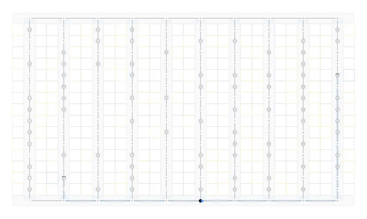
Watch the complete set of exact routes in Pickbench.
Table 20.3 compares their performance across the 10 workloads.
| Scenario | Distance (m) | Makespan (s) | Calculation (ms) | Valid / attempted |
|---|---|---|---|---|
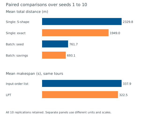
| S-shape | 2,329.8 (183.6) | 2,258.9 (177.0) | 3.80 | 10 / 10 |
| Exact | 1,949.0 (145.7) | 1,941.6 (144.0) | 6.66 | 10 / 10 |
Exact routing has a lower mean walking distance in these workloads. Both scenarios collect the same items, so their picking time is identical. Compare the reduction in walking with the calculation time shown in Table 20.3. An exact route cannot be longer than a feasible S-shape route for the same pick list. If your results suggest otherwise, check that both routes collect every requested item and return to the same depot.
Use the next animation to compare four methods on the same pick list. The warehouse in this illustration has 8 aisles and 10 storage positions per side. Each picker departs from the same I/O point and collects the same 3 orders, containing 13 items. Treat each picker as a separate routing alternative for the same work. The pick positions make the different route patterns easier to distinguish.
In the return method shown here, the picker enters each required aisle from the front and returns along it. Largest-gap routing serves intermediate aisles from their ends, leaving the longest pick-free stretches unwalked (de Koster et al. 2007, 495). Compare both with S-shape and exact routing. Use the method buttons to follow each picker, and open Inspect to check its stop sequence, order progress, and statistics.
Compare batching methods
Hold routing fixed at Ratliff-Rosenthal when comparing the batching rules. The single-order exact scenario supplies the reference without batching. Figure 20.2 shows the first savings-batch tour from seed 1. The animation replays all batches.
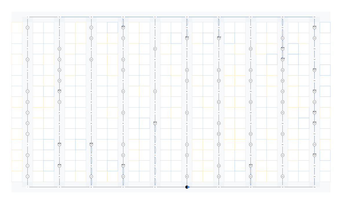
Table 20.4 compares the complete batched and single-order solutions. In the animation, follow one batch and notice how several orders share the same depot journey.
| Scenario | Distance (m) | Makespan (s) | Calculation (ms) | Valid / attempted |
|---|---|---|---|---|
| Exact | 1,949.0 (145.7) | 1,941.6 (144.0) | 6.66 | 10 / 10 |
| Seed batches | 761.7 (74.5) | 952.2 (88.6) | 3.04 | 10 / 10 |
| Savings batches | 693.1 (61.4) | 895.0 (78.6) | 110.64 | 10 / 10 |
Savings batching has the lowest mean travel distance of the 3 scenarios in Table 20.4. Collecting orders together reduces repeated depot journeys and aisle travel in this example. In an actual warehouse, the evaluation must also include sorting, order identification, cart design, and order completion requirements. Those activities are excluded from this teaching model and may change the practical recommendation.
Compare the schedules
Supply the same fixed tours to both schedulers. Changing the assignment leaves their total travel distance unchanged.
Figure 20.3 shows the tours assigned to each picker for seed 1. Play the animation and watch when each picker returns for another tour or finishes its last assignment. The shared clock lets you compare simultaneous work and idle periods.
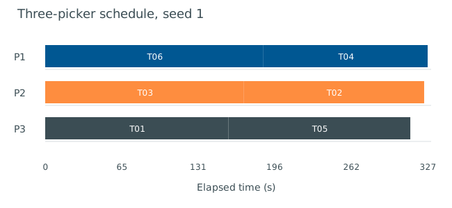
Table 20.5 compares the two assignments of the same tours.
| Scenario | Distance (m) | Makespan (s) | Calculation (ms) | Valid / attempted |
|---|---|---|---|---|
| List, 3 pickers | 693.1 (61.4) | 337.9 (17.3) | 0.22 | 10 / 10 |
| LPT, 3 pickers | 693.1 (61.4) | 322.5 (13.4) | 0.24 | 10 / 10 |
The two assignments have the same total distance and labor time because they use the same tours. LPT has a lower mean makespan in this experiment. Compare the final return times in Figure 20.3 to see how the tour assignments distribute the work.
Overall comparison
Figure 20.4 separates travel distance from completion time. The routing comparison changes the walk, the batching comparison changes order grouping, and the scheduling comparison changes work assignment. Keeping these decisions separate makes their effects easier to explain.
Capacity sensitivity
Table 20.6 varies carrying capacity while keeping the warehouse, seed-1 demand, routing method, batching rule, and picker count fixed.
| Capacity (items) | Tours | Distance (m) | Labor (s) | Makespan (s) |
|---|---|---|---|---|
| 10 | 12 | 1240.0 | 1375.33 | 1375.33 |
| 20 | 6 | 839.0 | 1041.17 | 1041.17 |
| 30 | 4 | 637.0 | 872.83 | 872.83 |
Increasing carrying capacity reduces the number of tours and the walking distance in these 3 cases. The calculation keeps walking speed and picking time fixed. Check that the larger load is practical with the available equipment before using the same assumption in a warehouse.
Applying the model
For WH-AS4 - Order-picking improvement, replace the synthetic inputs with the group’s cleaned SPR orders and location data. Establish the current picking process and document the facts, assumptions, and missing inputs relevant to the proposed change.
For the picking-only comparison, retain the current storage assignment, layout, and equipment. Generate feasible routes for the selected orders or batches. The single-block routing methods apply only where the warehouse geometry and movement rules satisfy their assumptions. Use a suitable graph-routing method when the actual aisle network differs.
When comparing combined interventions, check access, capacity, equipment, staffing, replenishment, and order completion. A different layout, product assignment, or type of equipment can require a different picking method. The assignment also permits a suitable travel model when generating detailed routes is impractical.
Estimate relevant setup, search, picking, sorting, unloading, and waiting times from case evidence or justified assumptions. Report the resource requirements alongside performance. The scheduling comparison assumes that pickers work independently. Check congestion and shared resources before using that assumption in SPR.
Use matched demand and evaluation conditions for each comparison. Explain the picking-only effect separately from combined storage, layout, equipment, and picking effects. Base the recommendation on feasibility, performance, resource trade-offs, and sensitivity results.
TipRun the Python example
Download the Python worked example, extract it, and open a terminal in its folder. The example uses Python 3.11 or later.
The commands repeat the experiments with the same saved orders and check the solutions. The replication table, summary table, and complete report are also available separately. To investigate capacity, change the carrying limit while keeping the orders and routing method fixed. Check that every order is collected once, every tour returns to the depot, and each picker carries a feasible load.
References
Graham, R. L. 1966. “Bounds for Certain Multiprocessing Anomalies.” Bell System Technical Journal 45 (9): 1563–81. https://doi.org/10.1002/j.1538-7305.1966.tb01709.x.
Graham, R. L. 1969. “Bounds on Multiprocessing Timing Anomalies.” SIAM Journal on Applied Mathematics 17 (2): 416–29. https://doi.org/10.1137/0117039.
Hall, Randolph W. 1993. “DISTANCE APPROXIMATIONS FOR ROUTING MANUAL PICKERS IN A WAREHOUSE.” IIE Transactions 25 (4): 76–87. https://doi.org/10.1080/07408179308964306.
Koster, M. B. M. de, E. S. van der Poort, and M. Wolters. 1999. “Efficient Orderbatching Methods in Warehouses.” International Journal of Production Research 37 (7): 1479–504. https://doi.org/10.1080/002075499191094.
Koster, René de, Tho Le-Duc, and Kees Jan Roodbergen. 2007. “Design and Control of Warehouse Order Picking: A Literature Review.” European Journal of Operational Research 182 (2): 481–501. https://doi.org/10.1016/j.ejor.2006.07.009.
Ratliff, H. Donald, and Arnon S. Rosenthal. 1983. “Order-Picking in a Rectangular Warehouse: A Solvable Case of the Traveling Salesman Problem.” Operations Research 31 (3): 507–21. https://doi.org/10.1287/opre.31.3.507.