Warehouse storage optimization

Aims

This tutorial introduces the concepts of warehouse storage optimization through mathematical modeling and analysis. The worked examples cover storage location allocation and capacity requirements under dedicated and randomized storage policies.

Learning Objectives

After completing this tutorial, you will be able to:

Develop a mathematical optimization model for the classical storage location assignment problem (SLAP).
Compare space utilization between dedicated and randomized storage policies.

Using the code

All code is folded: click Show code to expand a cell. The helper plot_warehouse_layout is defined in scripts/wh_plot_grid_layout_with_ios.py, and the input tables are saved to the data/ folder so that the solution can read them back.

Storage Location Assignment

Consider the warehouse layout shown in Figure 15.1. There are three I/O points through which four items enter and leave the warehouse. All three I/O points are located on the periphery of the building, with the first equidistant from storage spaces 14 and 15, the second from 5 and 9, and the third from storage spaces 2 and 3.

Show code

"""
(y)
↑
|   ╔═══════╦═════ IO3 ═════╦═══════╗
4   ║   1   ║   2   ║   3   ║   4   ║
|   ╠═══════╬═══════╬═══════╬═══════╣
3   ║   5   ║   6   ║   7   ║   8   ║
|   IO2 ════╬═══════╬═══════╬═══════╣
2   ║   9   ║   10  ║   11  ║   12  ║
|   ╠═══════╬═══════╬═══════╬═══════╣
1   ║   13  ║   14  ║   15  ║   16  ║
|   ╚═══════╩═════ IO1 ═════╩═══════╝
0---*---1---*---2---*---3---*---4---*--> (x)

"""

# Create output directory
import os
out_dir = "data"
os.makedirs(out_dir, exist_ok=True)

io_point_positions = {
    1: (2.5, 0.5),
    2: (0.5, 2.5),
    3: (2.5, 4.5),
}

# Save I/O point positions
import pandas as pd

df_io_points = pd.DataFrame.from_dict(io_point_positions, orient="index", columns=["x", "y"])
df_io_points.index.name = "IO Point"
df_io_points.to_csv(f"{out_dir}/io-point-positions.csv")

plot_warehouse_layout(4, 4, io_point_positions)

Figure 15.1: Warehouse layout with three I/O points and 16 same-sized storage locations.

The number of storage spaces \(S_i\) required for each of the four items is given by Table 15.1.

Show code

import pandas as pd

# Define the data for storage spaces
storage_spaces_data = {
  "Item": ["A", "B", "C", "D"],
  "N. of Storage Spaces": [3, 5, 2, 6],
}

# Create a DataFrame
df_storage_spaces = pd.DataFrame(storage_spaces_data).set_index("Item")

# To csv
df_storage_spaces.to_csv(f"{out_dir}/items-num-storage-spaces.csv")

# Display the math symbols in table
from IPython.display import Markdown, display
display(Markdown(df_storage_spaces.to_markdown()))

Table 15.1: Number of storage spaces \(S_{i}\) required for each item \(i\) totaling 16 spaces.

Item	N. of Storage Spaces
A	3
B	5
C	2
D	6

The frequency \(f_{ik}\) of trips for each item \(i\) and I/O point \(k\) and the cost \(c_{ik}\) of moving a unit load of item \(i\) to/from I/O point \(k\) are given in Table 15.2 and Table 15.3, respectively.

Show code

# Frequency of trips $f_{ik}$ for each item-I/O point $k$ combination
import pandas as pd

frequency_data = {
  "Item": ["A", "B", "C", "D"],
  "1": [150, 60, 96, 175],
  "2": [25, 200, 15, 135],
  "3": [88, 150, 85, 90],
}

df_frequency = pd.DataFrame(frequency_data).set_index("Item")
df_frequency.columns.name = "IO Point"

# To csv
df_frequency.to_csv(f"{out_dir}/frequency-items-io-points.csv")

df_frequency

Table 15.2: Frequency of trips \(f_{ik}\) for each item–I/O point combination.

IO Point	1	2	3
Item
A	150	25	88
B	60	200	150
C	96	15	85
D	175	135	90

Show code

# Cost $c_{ik}$ of moving a unit load of item $i$ to/from I/O point $k$
cost_data = {
  "Item": ["A", "B", "C", "D"],
  "1": [6, 7, 4, 15],
  "2": [5, 3, 7, 8],
  "3": [5, 6, 9, 12],
}

df_cost = pd.DataFrame(cost_data).set_index("Item")
df_cost.columns.name = "IO Point"

# To csv
df_cost.to_csv(f"{out_dir}/cost-moving-items-to-io-points.csv")

df_cost

Table 15.3: Cost \(c_{ik}\) of moving a unit load of item \(i\) to/from I/O point \(k\).

IO Point	1	2	3
Item
A	6	5	5
B	7	3	6
C	4	7	9
D	15	8	12

We assume that the costs are influenced by the handling requirements of each item. These requirements may include factors such as weight, volume, and fragility, which can affect the type of equipment needed or the labor intensity involved.

Our goal is to determine the optimal allocation of the four items to the 16 storage spaces such that the total travel cost between the I/O points and the storage spaces is minimized.

Distance Matrix and Weights

To calculate the distance matrix and weights, we follow these steps:

Distance Matrix: Compute the Manhattan distances \(d_{kj}\) between each I/O point \(k\) and storage location \(j\). The storage locations are arranged in a 2D grid, and their coordinates correspond to their centroids. For example:
- Storage location 1 is at \((1, 4)\).
- I/O point IO1 is at \((2.5, 0.5)\).
Use the formula for Manhattan distance: \[ d_{kj} = |x_k - x_j| + |y_k - y_j| \] where \((x_k, y_k)\) and \((x_j, y_j)\) are the coordinates of the I/O point and storage location, respectively.
Weights Calculation: Using the distance matrix, calculate the weights \(w_{ij}\) for each item \(i\) and storage location \(j\): \[ w_{ij} = \frac{\sum_{k=1}^{3} c_{ik} f_{ik} d_{kj}}{S_i} \] Here:
- \(c_{ik}\) is the cost of moving a unit load of item \(i\) to/from I/O point \(k\).
- \(f_{ik}\) is the frequency of trips for item \(i\) to/from I/O point \(k\).
- \(d_{kj}\) is the distance between I/O point \(k\) and storage location \(j\).
- \(S_i\) is the total number of storage spaces required for item \(i\).

Distance Matrix and Travel Time Models

For simplicity, we assume no batching occurs during the picking process. Therefore, the travel time is directly proportional to the distance between I/O points and storage locations.

If batching were considered, the travel time would depend on the sequence and combination of storage locations visited during a single picking route. This would require a more complex travel time model, such as those used in routing problems, to account for the additional travel time incurred when picking items from multiple storage locations.

Assumptions and Approach

First, for clarity, we restate our assumptions:

We assume a \(4\times4\) grid layout with three I/O points and four items.
Each item \(i\) has a specific number of slots \(S_i\) it requires.
The flow of items to I/O points is characterized by trip frequencies \(f_{ik}\) and unit handling costs \(c_{ik}\).
The sum of all \(S_i\) must equal the total number of available slots in the warehouse (no overloading or underutilization).

Unused storage locations

The last assumption (exact packing, \(\sum_i S_i = |J|\)) keeps this example small. When the number of available locations exceeds \(\sum_i S_i\), the location constraint becomes \(\sum_i x_{ij} \le 1\).

Our approach is as follows:

We compute the Manhattan distance \(d_{kj}\) between each I/O point \(k\) and storage location \(j\).
Using the Manhattan distances, we construct a weighted cost matrix \(w_{ij}\) that incorporates both the distance and the flow/cost parameters.
The model assigns exactly \(S_i\) slots per item, spreads them over the closest locations in terms of the weighted distance \(w_{ij}\), and balances across I/O patterns through \(f_{ik}\) and \(c_{ik}\).
The reported objective value is the total weighted travel burden across all slots.
If Gurobi is available, we solve the MILP directly. Otherwise, we expand items by their required slots and run an exact assignment on a \(16\times16\) cost matrix, which returns the same optimum for this structure.

Loading Data and Sanity Checks

It is good practice to load data so your model can adapt to changes in input without requiring code modifications.

Show code

# Load baseline inputs that you already saved earlier

import numpy as np
import pandas as pd

# Read IO points (already exported earlier)
io_points_df = pd.read_csv(f"{out_dir}/io-point-positions.csv", index_col="IO Point")
io_points = {int(k): (float(row["x"]), float(row["y"])) for k, row in io_points_df.iterrows()}
io_points_ids = sorted(io_points.keys())  # stable order

# Storage space requirements S_i
df_items_num_storage = pd.read_csv(f"{out_dir}/items-num-storage-spaces.csv", index_col="Item")
S = df_items_num_storage["N. of Storage Spaces"].to_dict()
items = list(S.keys())

# Frequencies f_{ik}
F = pd.read_csv(f"{out_dir}/frequency-items-io-points.csv", index_col="Item")
F.columns.name = "IO"

# Costs c_{ik}
C = pd.read_csv(f"{out_dir}/cost-moving-items-to-io-points.csv", index_col="Item")
C.columns.name = "IO"

# Grid shape
rows, cols = 4, 4

Next, to make sure our assumptions hold, we perform some sanity checks:

Show code

# Sanity checks, fail fast if something is off

# Grid capacity must match sum of S_i (we assume exact packing)
assert rows * cols == sum(S.values()), "Grid capacity does not match sum of S_i."

# Item sets must match across all tables
assert set(F.index) == set(items) == set(C.index), "Item sets differ across tables."

# IO sets must match across all tables
assert set(F.columns.astype(str)) == set(C.columns.astype(str)) == set(map(str, io_points_ids)), "IO sets mismatch."

Calculating Distances \(d_{kj}\) for IO-Location Pairs

For Manhattan distance

\[ d_{kj}=\lvert x_k-x_j\rvert+\lvert y_k-y_j\rvert, \]

we map location indices \(j\in\{1,\dots,16\}\) to integer cell centroids (Table 15.4):

Show code

from typing import Tuple
Coord = Tuple[float, float]


def index_to_xy(
    j: int,
    rows: int,
    cols: int,
    origin_top_left: bool = True,
) -> Tuple[int, int]:
    """
    Convert 1-based cell index j to integer grid coordinates (x, y).

    Numbering is row-major. With origin_top_left=True, index 1 is top-left.
    Otherwise, index 1 is bottom-left.

    Returns (x, y) with x, y in {1, 2, ..., cols/rows}.
    """
    if not (1 <= j <= rows * cols):
        raise ValueError(f"Index {j} is out of range 1..{rows * cols}.")

    x = (j - 1) % cols + 1
    row_idx = (j - 1) // cols  # 0-based row
    if origin_top_left:
        y = rows - row_idx
    else:
        y = row_idx + 1
    return x, y

# Precompute all (x,y) coordinates for locations
location_coords = {
    j: index_to_xy(j, rows, cols)
    for j in range(1, rows * cols + 1)}

df_location_coords = pd.DataFrame.from_dict(location_coords, orient="index", columns=["x", "y"])

df_location_coords

Table 15.4: Location coordinates (x, y) for each grid cell.

	x	y
1	1	4
2	2	4
3	3	4
4	4	4
5	1	3
6	2	3
7	3	3
8	4	3
9	1	2
10	2	2
11	3	2
12	4	2
13	1	1
14	2	1
15	3	1
16	4	1

Then, we compute the distance matrix \(d_{kj}\) from I/O points \(k\) to locations \(j\) using the Manhattan metric (Table 15.5):

Show code

import pandas as pd
def manhattan(p, q):
    return abs(p[0] - q[0]) + abs(p[1] - q[1])

d = pd.DataFrame(
    {
        k: [manhattan(io_points[k], index_to_xy(j, rows, cols, origin_top_left=True))
            for j in range(1, rows * cols + 1)]
        for k in io_points_ids
    },
    index=pd.Index(range(1, rows * cols + 1), name="Location(j)"),
)
d.columns = pd.Index(io_points_ids, name="IO Point(k)")
d

Table 15.5: Distance matrix \(d_{kj}\) from IO points \(k\) to locations \(j\) (Manhattan metric).

IO Point(k)	1	2	3
Location(j)
1	5.0	2.0	2.0
2	4.0	3.0	1.0
3	4.0	4.0	1.0
4	5.0	5.0	2.0
5	4.0	1.0	3.0
6	3.0	2.0	2.0
7	3.0	3.0	2.0
8	4.0	4.0	3.0
9	3.0	1.0	4.0
10	2.0	2.0	3.0
11	2.0	3.0	3.0
12	3.0	4.0	4.0
13	2.0	2.0	5.0
14	1.0	3.0	4.0
15	1.0	4.0	4.0
16	2.0	5.0	5.0

Computing Weights \(w_{ij}\) for Item-Location Pairs

We aggregate across I/O points, then normalize by the number of slots the item requires (Table 15.6):

\[ w_{ij} \;=\; \frac{\sum_{k} c_{ik}\,f_{ik}\,d_{kj}}{S_i}. \]

Show code

w = pd.DataFrame(
    0.0,
    index=pd.Index(range(1, rows * cols + 1), name="Location(j)"),
    columns=pd.Index(items, name="Item(i)"),
)

for i in items:
    for j in range(1, rows * cols + 1):
        agg = 0.0
        for k in io_points_ids:
            agg += C.loc[i, str(k)] * F.loc[i, str(k)] * d.loc[j, k]
        w.loc[j, i] = agg / S[i]

# Show with 2 decimals and add thousands separator
w.round(2).map(lambda x: f"{x:,.2f}")

Table 15.6: Weights \(w_{ij}\) reflecting average travel burden per slot for item \(i\) at location \(j\).

Item(i)	A	B	C	D
Location(j)
1	1,876.67	1,020.00	1,830.00	2,907.50
2	1,471.67	876.00	1,308.00	2,470.00
3	1,513.33	996.00	1,360.50	2,650.00
4	2,001.67	1,380.00	1,987.50	3,447.50
5	1,681.67	996.00	1,968.00	2,470.00
6	1,276.67	852.00	1,446.00	2,032.50
7	1,318.33	972.00	1,498.50	2,212.50
8	1,806.67	1,356.00	2,125.50	3,010.00
9	1,528.33	1,092.00	2,158.50	2,212.50
10	1,123.33	948.00	1,636.50	1,775.00
11	1,165.00	1,068.00	1,689.00	1,955.00
12	1,653.33	1,452.00	2,316.00	2,752.50
13	1,416.67	1,308.00	2,401.50	2,135.00
14	1,011.67	1,164.00	1,879.50	1,697.50
15	1,053.33	1,284.00	1,932.00	1,877.50
16	1,541.67	1,668.00	2,559.00	2,675.00

Optimizing SLAP

We solve

\[ \min \sum_{i}\sum_{j} w_{ij}\,x_{ij} \]

subject to

\[ \sum_{i} x_{ij}=1\;\;(\forall j), \qquad \sum_{j} x_{ij}=S_i\;\;(\forall i), \qquad x_{ij}\in\{0,1\}. \]

Table 15.7 shows the resulting assignment. If Gurobi is not available, the code falls back to SciPy’s linear assignment (Hungarian algorithm).

Show code

assignment = {}
objective_value = None
solver_used = None

try:

    # If Gurobi is available, use it
    import gurobipy as gp
    from gurobipy import GRB

    # Suppress Gurobi license messages
    gp.setParam("LogToConsole", 0)
    gp.setParam("OutputFlag", 0)

    m = gp.Model("SLAP")
    x = m.addVars(items, range(1, rows * cols + 1), vtype=GRB.BINARY, name="x")

    # Each location used once
    for j in range(1, rows * cols + 1):
        m.addConstr(sum(x[i, j] for i in items) == 1)

    # Each item occupies S_i slots
    for i in items:
        m.addConstr(
            sum(x[i, j]
            for j in range(1, rows * cols + 1)) == S[i])

    # Objective
    m.setObjective(
        sum(w.loc[j, i] * x[i, j]
        for i in items
        for j in range(1, rows * cols + 1)),
        GRB.MINIMIZE)

    m.Params.OutputFlag = 0
    m.optimize()

    objective_value = float(m.objVal)
    for j in range(1, rows * cols + 1):
        for i in items:
            if x[i, j].X > 0.5:
                assignment[j] = i
    solver_used = "Gurobi MILP"

# Scipy is a free alternative
except Exception:
    # Exact fallback using the linear assignment on expanded items
    from scipy.optimize import linear_sum_assignment

    # Expand items based on their required slots
    expanded = []
    for i in items:
        expanded.extend([i] * S[i])

    # Create the cost matrix for the assignment problem
    cost = np.zeros((rows * cols, rows * cols))
    for r, i in enumerate(expanded):
        for j in range(1, rows * cols + 1):
            cost[r, j - 1] = w.loc[j, i]

    # Solve the assignment problem using the Hungarian algorithm
    r_idx, c_idx = linear_sum_assignment(cost)
    objective_value = float(cost[r_idx, c_idx].sum())

    # Map the assignment results back to the original locations
    for r, c in zip(r_idx, c_idx):
        assignment[c + 1] = expanded[r]

    solver_used = "Hungarian fallback"

# Create a DataFrame for the assignment results
assign_df = pd.Series(assignment, name="Item(i)")

# Map the assignment results back to the original locations
assign_df = assign_df.rename_axis("Location(j)").sort_index().to_frame()
assign_df

Table 15.7: Optimal assignment of items \(i\) to locations \(j\).

	Item(i)
Location(j)
1	B
2	C
3	C
4	B
5	B
6	B
7	A
8	B
9	D
10	D
11	D
12	A
13	D
14	D
15	D
16	A

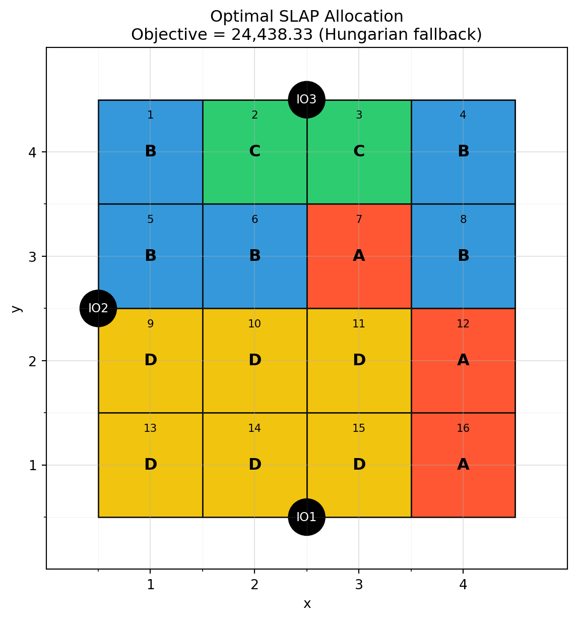
We map each location to its item label, and we color slots by item for readability (Figure 15.2).

Show code

# Color palette per item
color_map = {"A": "#FF5733", "B": "#3498DB", "C": "#2ECC71", "D": "#F1C40F"}

# Build a cell-indexed facecolor map from the item assignment
cell_colors = {j: color_map[assignment[j]] for j in assignment}

fig, ax = plot_warehouse_layout(
    rows=rows,
    cols=cols,
    io_positions=io_points,
    labels=assignment,                      # center letters A,B,C,D
    colors=cell_colors,                     # facecolors by item
    origin_top_left=True,
    annotate_cell_index=True,               # light grid index reference
    annotate_user_label=True,
    title=f"Optimal SLAP Allocation\nObjective = {objective_value:,.2f} ({solver_used})",
)

Figure 15.2: Optimal SLAP allocation drawn on the \(4\times4\) grid with I/O points.

Space Allocation: Random vs. Dedicated Policies

A unit-load warehouse specializing in five high-turnover consumer items is scheduled to receive the quantities shown in Table 15.8 for the next 12 periods.

Show code

import pandas as pd

# Define the data for scheduled receipts
data = {
  "Period": [1, 2, 3, 4, 5, 6, 7, 8, 9, 10, 11, 12],
  "A": [20, 15, 30, 12, 14, 60, 17, 20, 21, 22, 23, 23],
  "B": [12, 8, 4, 6, 7, 1, 12, 40, 13, 12, 12, 12],
  "C": [66, 15, 16, 17, 18, 19, 15, 16, 17, 18, 19, 15],
  "D": [22, 22, 25, 21, 18, 14, 23, 36, 30, 22, 89, 22],
  "E": [97, 12, 88, 66, 79, 55, 9, 25, 96, 90, 90, 88],
}

# Create a DataFrame
df_scheduled_receipts = pd.DataFrame(data).set_index("Period")
df_scheduled_receipts.to_csv(f"{out_dir}/scheduled_receipts.csv")
df_scheduled_receipts

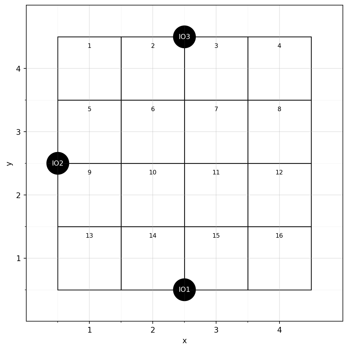
Table 15.8: Scheduled receipts for five items (A, B, C, D, and E) throughout the 12 periods.

	A	B	C	D	E
Period
1	20	12	66	22	97
2	15	8	15	22	12
3	30	4	16	25	88
4	12	6	17	21	66
5	14	7	18	18	79
6	60	1	19	14	55
7	17	12	15	23	9
8	20	40	16	36	25
9	21	13	17	30	96
10	22	12	18	22	90
11	23	12	19	89	90
12	23	12	15	22	88

The warehouse manager likes to maintain a quantity of safety stock for each product in each period equal to 10% of the scheduled receipt of that product for the next period. We determine the total storage spaces required under the dedicated and random storage policies considering the following assumptions:

Blockage is allowed (i.e., products can be stored in front of each other).
The products have the same dimensions and handling requirements.
Inventory is not carried over between periods.
Safety stock is calculated as a fixed percentage (viz., 10%) of the next period’s receipt (rounded up).

Safety Stock Rule

More formally, the safety stock in period \(t\) equals a fraction \(\alpha\) (viz., 10%) of the next period’s receipt:

\[ \text{SS}_{i,t}=\alpha \cdot \text{receipt}_{i,t+1}. \]

Required spaces are rounded up to integer slots:

\[ \text{req}_{i,t}=\left\lceil \text{receipt}_{i,t} + \text{SS}_{i,t} \right\rceil = \left\lceil \text{receipt}_{i,t} + \alpha \cdot \text{receipt}_{i,t+1} \right\rceil. \]

For the last period we set \(\text{receipt}_{i,T+1}=0\).

Loading Data

Show code

import numpy as np
import pandas as pd
import matplotlib.pyplot as plt

# Load scheduled receipts (rows = Period, columns = items)
df_sched = pd.read_csv(f"{out_dir}/scheduled_receipts.csv", index_col="Period")

df_sched

Listing 15.1

	A	B	C	D	E
Period
1	20	12	66	22	97
2	15	8	15	22	12
3	30	4	16	25	88
4	12	6	17	21	66
5	14	7	18	18	79
6	60	1	19	14	55
7	17	12	15	23	9
8	20	40	16	36	25
9	21	13	17	30	96
10	22	12	18	22	90
11	23	12	19	89	90
12	23	12	15	22	88

Computing Safety Stock and Required Spaces

We implement the formula above with a one-step forward shift to obtain \(\text{receipt}_{i,t+1}\) (Table 15.9).

Show code

# Safety Constants
ALPHA_SAFETY = 0.1

# Next period receipts (fill 0 at the end)
next_receipt = df_sched.shift(-1, fill_value=0)

# Safety stock rule: SS_{i,t} = α * receipt_{i,t+1}
ss = ALPHA_SAFETY * next_receipt

# Period requirements: req_{i,t} = ceil(receipt_{i,t} + SS_{i,t})
req = np.ceil(df_sched + ss).astype(int)

req

Table 15.9: Expected required space per period considering safety stock of 10%.

	A	B	C	D	E
Period
1	22	13	68	25	99
2	18	9	17	25	21
3	32	5	18	28	95
4	14	7	19	23	74
5	20	8	20	20	85
6	62	3	21	17	56
7	19	16	17	27	12
8	23	42	18	39	35
9	24	15	19	33	105
10	25	14	20	31	99
11	26	14	21	92	99
12	23	12	15	22	88

Sizing Capacity for Different Storage Policies

Dedicated reserves capacity item by item. Therefore, for each item \(i\) we find the peak requirement across all periods, then sum these peaks:

\[ \text{Cap}^{\text{ded}}=\sum_{i}\max_{t}\text{req}_{i,t}. \]

Table 15.10 shows the per-item peaks and the total required spaces by the Dedicated policy.

Show code

# Per-item peak across periods, used by Dedicated policy
per_item_max = req.max(axis=0)

# Dedicated capacity: sum of item-wise peaks
dedicated_spaces = int(per_item_max.sum())

per_item_max.to_frame(name="Peak Requirement")

Table 15.10: Dedicated storage capacity requirements (spaces in unit slots). For each item, the peak requirement across all periods is used by the Dedicated policy.

	Peak Requirement
A	62
B	42
C	68
D	92
E	105

Random pools capacity across all items. Therefore, for each period \(t\) we find the total requirement across all items, then take the peak of these totals:

\[ \text{Cap}^{\text{rnd}}=\max_{t}\sum_{i}\text{req}_{i,t}. \]

Table 15.11 shows the per-period totals and the total required spaces by the Random policy.

Show code

# Calculate total requirements per period
total_per_period = req.sum(axis=1)
# Random capacity: peak of total requirements across periods
random_spaces = int(total_per_period.max())

total_per_period.to_frame(name="Total Requirement")

Table 15.11: Random storage capacity requirements (spaces in unit slots). For each period, the total requirement across all items is used by the Random policy.

	Total Requirement
Period
1	227
2	90
3	178
4	137
5	153
6	159
7	91
8	157
9	196
10	189
11	252
12	160

Hence,

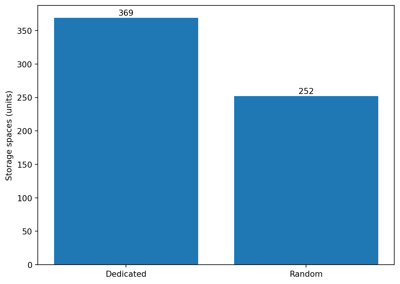
Dedicated requires \(\sum_i \max_t \text{req}_{i,t} = \mathbf{369}\) spaces.
Random requires \(\max_t \sum_i \text{req}_{i,t} = \mathbf{252}\) spaces.

Figure 15.3 compares the two policies in terms of required spaces.

Show code

fig = plt.figure()
bars = plt.bar(["Dedicated", "Random"], [dedicated_spaces, random_spaces])
plt.ylabel("Storage spaces (units)")

# Annotate the bars with their respective values
for bar in bars:
    height = bar.get_height()
    plt.text(bar.get_x() + bar.get_width() / 2, height + 1, f"{height}", ha="center", va="bottom")

plt.tight_layout()
plt.show()

Figure 15.3: Capacity sizing under Dedicated and Random policies (spaces in unit slots).

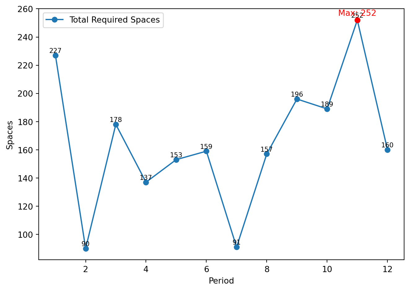
Figure 15.4 shows the total required spaces by period, highlighting the pooling peak that drives the Random policy.

Show code

fig = plt.figure()
plt.plot(total_per_period.index, total_per_period.values, marker="o", label="Total Required Spaces")
plt.xlabel("Period")
plt.ylabel("Spaces")

# Annotate each point
for x, y in zip(total_per_period.index, total_per_period.values):
    plt.text(x, y + 1, f"{y}", ha="center", va="bottom", fontsize=8)

# Highlight the maximum point
max_period = total_per_period.idxmax()
max_value = total_per_period.max()
plt.scatter(max_period, max_value, color="red", zorder=5)
plt.text(max_period, max_value + 2, f"Max: {max_value}", ha="center", va="bottom", fontsize=10, color="red")

plt.legend()
plt.tight_layout()
plt.show()

Figure 15.4: Total required spaces by period, showing the pooling peak that drives the Random policy.