Practice questions
These are examples of questions that could appear on the exam. On the exam, questions presented here in open form will have multiple-choice alternatives from which you select the expected answer.
Multiple-choice questions
M1 Facility location
A facility location formulation is given below. Let \(I\) be the set of candidate facility locations and \(J\) the set of demand nodes.
\[ \begin{aligned} \min\quad &\sum_{i\in I}\sum_{j\in J}h_jd_{ij}x_{ij}\\ \text{subject to}\quad &\sum_{i\in I}x_{ij}=1 &&\forall j\in J,\\ &\sum_{i\in I}y_i=p,\\ &x_{ij}\leq y_i &&\forall i\in I,\ j\in J,\\ &x_{ij},y_i\in\{0,1\} &&\forall i\in I,\ j\in J. \end{aligned} \]
Here \(h_j\) is the weight of demand node \(j\), and \(d_{ij}\) is the shortest distance between demand node \(j\) and facility location \(i\). The \(x_{ij}\) variables assign demand nodes to facilities, and the \(y_i\) variables indicate facility openings. Which type of problem does this formulation describe?
- P-median
- P-center
- Fixed charge
- None of the above
NoteSolution
Answer A.
The model opens exactly \(p\) facilities and minimizes the sum of demand-weighted assignment distances. These features define the p-median formulation. Each demand node is assigned to one facility, and \(x_{ij}\leq y_i\) permits assignment only to an open facility.
A p-center objective minimizes the largest service distance. A fixed-charge formulation includes facility-opening costs in the objective.
Numerical illustration.
- Read the inputs for this separate example. Open \(p=\) 2 facilities using the distances in Table 29.1 and the demand weights in Table 29.2. The distance rows identify candidate facilities, and the columns identify demand nodes.
| Facility | 1 | 2 | 3 |
|---|---|---|---|
| 1 | 0 | 4 | 7 |
| 2 | 4 | 0 | 3 |
| 3 | 7 | 3 | 0 |
| Demand node | Demand weight |
|---|---|
| 1 | 2 |
| 2 | 3 |
| 3 | 1 |
- Use the optimal facility assignment. Opening facilities 1, 2 gives the optimal assignments in Table 29.3. Their total demand-weighted distance is 3.
| Demand node | Facility | Distance | Demand weight | Weighted distance |
|---|---|---|---|---|
| 1 | 1 | 0 | 2 | 0 |
| 2 | 2 | 0 | 3 | 0 |
| 3 | 2 | 3 | 1 | 3 |
M2 Assignment variables
Suppose the \(x\) variables in M1 Facility location are continuous between 0 and 1. Demand is divisible, and the model describes a deterministic allocation of demand. What does \(x_{ij}\) represent in this model?
- Probability of demand node \(j\) being assigned to facility \(i\)
- Probability of demand node \(j\) not being assigned to facility \(i\)
- Fraction of demand at node \(j\) assigned to facility \(i\)
- None of the above
NoteSolution
Answer C.
Relaxing the assignment variables permits fractional allocations. The fractions for each demand node must still sum to 1. The facility-opening variables remain binary under the stated relaxation.
For example, \(x_{1j}=\) 0.4 and \(x_{2j}=\) 0.6 allocate demand to two open facilities. The facilities receive 40% and 60% of node \(j\)’s demand, respectively. These values are deterministic shares of divisible demand.
Table 29.4 shows the feasible allocation for one unit of normalized demand. Fractional allocation is permitted, but an optimal solution need not split demand.
| Facility | Open | Fraction of demand | Percentage of demand | Allocated demand |
|---|---|---|---|---|
| 1 | 1 | 0.40 | 40.00 | 0.40 |
| 2 | 1 | 0.60 | 60.00 | 0.60 |
M3 Order-picking methods
Using the order-picking terminology in de Koster et al., which statement is correct?
- Zoning can be applied in a parts-to-picker system.
- Batch picking restricts every picking route to items from a single SKU.
- Wave picking is used if orders for a common destination are released sequentially for picking in multiple warehouse areas.
- All of the above statements are correct.
NoteSolution
Answer A. The alternatives describe different ways to organize picking:
- Zoning divides a picking area into zones and can be used in a parts-to-picker system. Kardex’s automated-storage picking zones use carousels and other systems that deliver stored items to operators.
- Picking by article, or batch picking, combines multiple customer orders in one picking process. A batch can contain several SKUs.
- In the course’s wave-picking definition, orders for a common destination are released simultaneously across warehouse areas (Koster et al. 2007, 484, 485). The word “sequentially” therefore makes C false.
M4 Fire-station coverage
A rural county administration is considering five locations for fire stations. The county has five population zones, and each zone must be within 15 minutes of a station. In Table 29.5, 1 means a station is within 15 miles of a zone, and 0 means it is farther away. The average emergency speed is 60 miles per hour, so the distance and time limits agree.
| Population zone | Site 1 | Site 2 | Site 3 | Site 4 | Site 5 |
|---|---|---|---|---|---|
| 1 | 1 | 1 | 0 | 0 | 0 |
| 2 | 1 | 1 | 1 | 0 | 0 |
| 3 | 0 | 1 | 0 | 1 | 1 |
| 4 | 0 | 0 | 1 | 0 | 1 |
| 5 | 0 | 0 | 1 | 1 | 0 |
| Opening cost ($1,000) | 90 | 70 | 110 | 50 | 50 |
Apply the weighted greedy set-covering rule used in class. At each iteration, select the site with the smallest opening cost per newly covered zone. Which location is not selected?
- 2
- 3
- 4
- 5
NoteSolution
Answer B, location 3.
Apply the weighted greedy rule by dividing each opening cost by the number of zones it newly covers. The initial ratios are shown in Table 29.6. Opening costs are in dollars, and ratios are dollars per newly covered zone.
| Site | Opening cost ($) | Initially covered zones | Cost per initially covered zone ($) |
|---|---|---|---|
| 1 | 90,000.00 | 2 | 45,000.00 |
| 2 | 70,000.00 | 3 | 23,333.33 |
| 3 | 110,000.00 | 3 | 36,666.67 |
| 4 | 50,000.00 | 2 | 25,000.00 |
| 5 | 50,000.00 | 2 | 25,000.00 |
Select site 2. It has the smallest initial ratio and covers zones 1, 2, 3. The remaining uncovered zones are 4, 5.
Recompute the cost per newly covered zone. Sites 4, 5 each cover one of the remaining zones for $50,000. The alternative site 3 covers both remaining zones for $110,000. The two lower-ratio sites are tied, so the greedy rule selects them in either order.
Both selection orders are shown in Table 29.7 and Table 29.8.
| Selection | Newly covered | Cost per new point (dollars) |
|---|---|---|
| 1. Site 2 | 1, 2, 3 | 23,333.33 |
| 2. Site 4 | 5 | 50,000.00 |
| 3. Site 5 | 4 | 50,000.00 |
| Selection | Newly covered | Cost per new point (dollars) |
|---|---|---|
| 1. Site 2 | 1, 2, 3 | 23,333.33 |
| 2. Site 5 | 4 | 50,000.00 |
| 3. Site 4 | 5 | 50,000.00 |
The selected set is {2, 4, 5}, with total opening cost $170,000.
M5 Forklift selection
A warehouse designer wants the lowest floor area per pallet position in a unit-load, single-deep storage system. Which forklift in Table 29.9 best contributes to that goal? Assume the warehouse can accommodate the stated clear heights, and the pallet and rack geometry is the same for all four options.
| Number | Forklift type | Clear height (ft) | Minimum aisle (in) | Levels |
|---|---|---|---|---|
| 1 | Counterbalanced | 21 | 144 | 4 |
| 2 | Reach-Fork Truck | 21 | 105 | 4 |
| 3 | Swing-Reach Truck | 21 | 66 | 4 |
| 4 | Transtacker (TRT) | 64 | 56 | 13 |
- 1
- 2
- 3
- 4
NoteSolution
Answer D, forklift 4.
Assumptions and notation.
All equipment options are assumed feasible, including their stated clear-height requirements. The selected option requires 64 ft of clear height.
Compare the storage footprint per pallet position. Equipment purchase cost, throughput, and other operating requirements are outside this comparison.
Let \(p\) be pallet width, \(s\) pallet spacer, \(r\) rack upright, \(l\) pallet length, \(f\) flue width, and \(a\) aisle width. All horizontal lengths are in inches and are equal across alternatives except for aisle width \(a\).
Let \(d\) be the dimensionless number of pallet positions deep per rack face, with \(d=\) 1 for single-deep storage. The storage unit has two back-to-back rack faces, with two pallet positions per face and level. For this single-deep unit with \(L\) levels, its width, depth, and number of pallet positions are
\[ W=2p+3s+r,\qquad D=2ld+f+a,\qquad P=4L. \]
The floor area per pallet position is
\[ \frac{WD}{144P} =\frac{(2p+3s+r)(2ld+f+a)}{576L} \quad\mathrm{ft}^2/\mathrm{position}. \]
The factor 144 converts square inches to square feet. Write \(C=2ld+f\) to compare alternatives using \((C+a)/L\). The common rack depth \(C\) is positive and remains in the numerator. The comparison expressions are shown in Table 29.10.
| Option | Aisle (in) | Levels | Comparison expression |
|---|---|---|---|
| 1 | 144 | 4 | \(\frac{C}{4} + 36\) |
| 2 | 105 | 4 | \(\frac{C}{4} + \frac{105}{4}\) |
| 3 | 66 | 4 | \(\frac{C}{4} + \frac{33}{2}\) |
| 4 | 56 | 13 | \(\frac{C}{13} + \frac{56}{13}\) |
Forklift 4 has both the narrowest aisle and the largest number of levels. For every positive common rack depth, its comparison expression is smaller than each alternative. Under the stated feasibility assumptions, it gives the smallest floor area per pallet position.
M6 Popularity profiles
In a warehouse, a minority of items typically generates most picking activity. A popularity profile, also called an ABC curve, shows the percentage of picks associated with the percentage of SKUs ranked by descending popularity. Using the picking-popularity measure and Frazelle’s illustrative grouping, which statement is false?
- A picking-popularity profile ranks SKUs by their total unit sales.
- Breakpoints in a popularity profile can define item families. For example, the top 5% of items, family A, may account for 50% of picking activity; the next 15%, family B, may bring the cumulative activity to 80%; and the remaining 80%, family C, account for the rest.
- Item families may suggest storage modes. Family A may use an automated, highly productive mode; B a semi-automated, moderately productive mode; and C a manual mode with high storage density.
- Family breakpoints may suggest locations within a storage mode. A items may occupy the golden zone, near a travel aisle and/or waist level; B items the silver zone; and C items the remaining spaces.
NoteSolution
Answer A. A picking-popularity profile ranks items by picking requests. One request can contain several units.
- A is false because total unit sales and picking requests are different measures.
- B gives an illustrative distribution. Its percentages are not fixed rules for every warehouse.
- C and D describe possible uses of the profile for storage-mode and location decisions.
Frazelle (2016, 56, 59) describes the principle of assigning the most popular items to the most accessible locations.
The cumulative shares for this illustrative grouping are calculated in Table 29.11.
M7 Storage policies
Consider a warehouse storing several SKUs. Each location holds one SKU at a time. Which statement about storage-assignment policies is false?
- In class-based storage, SKUs are grouped using a stated criterion, and an incoming load may use an available location within its assigned class region.
- In dedicated storage, locations remain reserved for a SKU even when that SKU is out of stock.
- Random storage permanently reserves predetermined locations for individual SKUs.
- With random storage, the system must keep track of the locations containing each SKU.
NoteSolution
Answer C. Random storage uses eligible empty locations without permanent reservations for individual SKUs.
- Dedicated storage reserves locations for a SKU, including when those locations are empty.
- Class-based storage groups SKUs and permits location sharing within each assigned class region.
- Random storage requires location records so stored items can be found (Koster et al. 2007, 488–90; Bahrami et al. 2019, 391).
Eligibility may depend on load size, temperature, or compatibility. Under the standard random-storage rule, each eligible empty location is equally likely to be selected (Koster et al. 2007, 488).
Permanent reservation alone does not guarantee the shortest travel (Bahrami et al. 2019, 391, 393–94).
M8 Dynamic-programming transitions
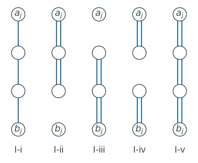
Consider the Ratliff and Rosenthal order-picking algorithm when at least one item must be picked in each aisle. The within-aisle configurations are shown in Figure 29.1, and the between-aisle configurations in Figure 29.2. The boundary vertices are \(a_j\) at the top and \(b_j\) at the bottom of aisle \(j\).
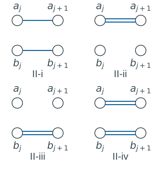
A state records the degrees of the two boundary vertices and the number of connected components of the partial tour. \(U\) denotes odd degree, \(E\) positive even degree, and 0 degree zero. The labels 1C and 2C denote one and two connected components. \(L_j^-\) is the state before adding aisle \(j\)’s within-aisle edges, and \(L_j^+\) is the state afterwards. The transition tables are Table 29.12 and Table 29.13. A blank cell denotes an infeasible transition. If a boundary vertex is itself required, a transition must also give it positive degree before that vertex leaves the boundary.
| Class | I-i | I-ii | I-iii | I-iv | I-v |
|---|---|---|---|---|---|
| (U, U, 1C) | (E, E, 1C) | A | (U, U, 1C) | (U, U, 1C) | (U, U, 1C) |
| (E, 0, 1C) | (U, U, 1C) | (E, 0, 1C) | (E, E, 2C) | (E, E, 2C) | (E, E, 1C) |
| (0, E, 1C) | (U, U, 1C) | (E, E, 2C) | (0, E, 1C) | (E, E, 2C) | (E, E, 1C) |
| (E, E, 1C) | (U, U, 1C) | (E, E, 1C) | (E, E, 1C) | (E, E, 1C) | (E, E, 1C) |
| (E, E, 2C) | (U, U, 1C) | (E, E, 2C) | (E, E, 2C) | (E, E, 2C) | (E, E, 1C) |
| Class | II-i | II-ii | II-iii | II-iv |
|---|---|---|---|---|
| (U, U, 1C) | (U, U, 1C) | B | ||
| (E, 0, 1C) | (E, 0, 1C) | (E, E, 2C) | ||
| (0, E, 1C) | (0, E, 1C) | (E, E, 2C) | ||
| (E, E, 1C) | (E, 0, 1C) | (0, E, 1C) | (E, E, 1C) | |
| (E, E, 2C) | (E, E, 2C) |
Which description of the missing cells A and B is correct?
- A is (U, U, 1C) and B is (E, 0, 1C).
- A is (U, 0, 1C) and B is (U, 0, 1C).
- A is (U, U, 1C) and B is infeasible because the old boundary vertices retain odd degrees.
- A is (U, 0, 1C) and B is (E, 0, 1C).
NoteSolution
Answer C.
Cell A is (U, U, 1C). Configuration I-ii adds a doubled path from the top boundary vertex. Both boundary degrees remain odd, and the partial tour still has one connected component.
Cell B is infeasible. Configuration II-ii moves the boundary using only a doubled top connection. The old top and bottom vertices retain odd degrees after they leave the boundary. Later aisle additions cannot repair those degrees, which makes the transition infeasible (Ratliff and Rosenthal 1983, 508–10).
M9 Smart warehouses
In the CPS framework used for this question, pickup, delivery, and bookkeeping are automated and paperless. Cyber-physical systems monitor physical processes and provide a virtual representation for control and decisions. Humans remain part of the framework, including instruction and monitoring roles. Using Liu et al.’s CPS components and Zhen and Li’s classification of smart-warehouse decisions, which statement is false?
- A CPS-based smart warehouse contains four main components, namely CPS devices, inventories, robots, and human beings.
- Sustainability goals can be pursued through operational decisions such as sequencing, scheduling, and power-load management.
- Basic smart-warehouse characteristics can be classified as information interconnection, equipment automation, process integration, and environmental sustainability.
- In Zhen and Li’s classification, equipment characteristics are associated with tactical decisions and product characteristics with operational decisions.
NoteSolution
Answer D. Zhen and Li associate equipment characteristics with strategic decisions and product characteristics with tactical decisions (Zhen and Li 2022, 32). Option D assigns both characteristics to the wrong decision level.
The other alternatives agree with the cited frameworks:
- Sequencing, scheduling, and power-load management are operational decisions. They can address environmental and operational objectives (Zhen and Li 2022, 48).
- Liu and colleagues identify CPS devices, inventories, robots, and human beings as the four components in A (Liu et al. 2018, 1–2).
- The basic characteristics in C use the framework named in the question.
M10 Storage assignment and travel
Consider the rectangular warehouse in Figure 29.3. The two parallel aisles are one distance unit apart, and each aisle has two pick locations one unit apart. The I/O point coincides with the southwest location. Each location holds exactly one SKU, and SKUs 1, 2, 3, and 4 have identical dimensions.
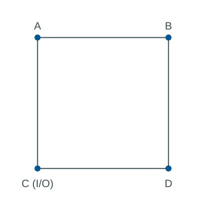
The annual orders are given in Table 29.14. Let \(N\) be an integer with \(N\geq2\). Each order is picked in one multi-command trip that starts and finishes at the I/O point. Orders are picked consecutively, and travel follows an optimal route for each order.
| Order set | Products | Times ordered |
|---|---|---|
| I | 1 | \(N\) |
| II | 2, 3, 4 | \(N+1\) |
What is the total travel distance under an optimal assignment of SKUs to locations?
- \(4N+4(N+1)\)
- \(4(N+1)\)
- \(2(N+1)\)
- \(4N\)
NoteSolution
Answer B.
The minimum total travel distance is \(4 \left(N + 1\right)\).
Assign SKU 1 to the I/O location C. Every order in set I then requires 0 distance units.
Assign the remaining SKUs to the other corners. A shortest closed trip through their locations follows the warehouse perimeter and has length 4. The order of those SKUs among the remaining corners does not affect the trip length.
The assignment and travel for each order set are shown in Table 29.15. The location labels refer to Figure 29.3.
| Order set | Products | Times ordered | Distance per trip | Pick locations | Annual distance |
|---|---|---|---|---|---|
| I | 1 | \(N\) | 0 | C | \(0\) |
| II | 2, 3, 4 | \(N + 1\) | 4 | A, B, D | \(4 \left(N + 1\right)\) |
Every order has its own closed trip, so the order-processing sequence does not change the total distance.
An order in set II visits 3 distinct corners under any assignment, including assignments that use the I/O corner. The trip spans both dimensions of the rectangle and has minimum length 4.
Placing SKU 1 at the I/O point attains that bound while minimizing travel for set I. Enumerating all 24 assignments gives 6 optimal assignments for the stated domain \(N\geq2\).
M11 Popularity profiles and storage modes
A popularity profile ranks SKUs by descending picking popularity and shows their cumulative share of picking activity. For Frazelle’s illustrative popularity-based grouping, which statement is false?
- Ranking SKUs by picking popularity can identify the items responsible for a large share of picking activity.
- Breakpoints in a popularity profile can define item families. For example, the top 5% of items, family A, may account for 50% of picking activity; the next 15%, family B, may bring the cumulative activity to 80%; and the remaining 80%, family C, account for the rest.
- Item families may suggest storage modes. Family A may use a manual mode with high storage density; B a semi-automated, moderately productive mode; and C an automated, highly productive mode.
- Family breakpoints may suggest locations within a storage mode. A items may occupy the golden zone, near a travel aisle and/or waist level; B items the silver zone; and C items the remaining spaces.
NoteSolution
Answer C. The stated grouping reverses the A and C storage-mode assignments in the cited example.
The example suggests these storage modes:
- Family
Amay use an automated, highly productive mode. - Family
Bmay use a semi-automated, moderately productive picking mode. - Family
Cmay use a manual picking mode with high storage density.
The grouping is illustrative. Storage-mode decisions also depend on pick density, storage requirements, and economics (Frazelle 2016, 62, 278–80).
A popularity profile measures picking activity. Production-volume P-Q analysis ranks production quantities. Both use an ABC-style ranking, and the passages under A distinguish their measures.
The following passages support the alternatives.
Option A.
P–Q analysis: The P–Q analysis, also referred to as “ABC” or “Pareto” analysis, sorts the parts in decreasing order of their production quantities (Figure 5.29). A major advantage of this analysis is that it allows the facility designer to focus efforts on reducing material handling costs, work-in-process (WIP) inventory, queuing times, production led times, and operating costs only on high-volume parts. (Heragu 2022, 128).
Item Popularity Profile
As mentioned earlier, a minority of the items in a warehouse typically generates a majority of the picking activity. The popularity profile (sometimes called an ABC curve or a Pareto distribution) indicates the x percent of picks associated with y percent of the SKUs (ranked by descending popularity). Figure 2.26 is a classic popularity profile indicating that the 10 percent most popular items yield 70 percent of the picking activity, the 50 percent most popular items yield 90 percent of the picking activity, and so on. (Frazelle 2016, 56)
Option B.
Key breakpoints in the distribution suggest delineations between item popularity families. For example, the top 5 percent of items (Family A) may make up 50 percent of the picking activity, the next 15 percent of items (Family B) may take us to 80 percent of the picking activity, and the remaining 80 percent of items (Family C) cover the remaining picking activity. (Frazelle 2016, 59)
Option C.
These families, in turn, may suggest three alternative storage modes—Family A in an automated, highly productive storage mode; Family B in a semi-automated, moderately productive picking mode; and Family C in a manual picking mode that offers high storage density. (Frazelle 2016, 59)
Option D.
The family breakpoints also may suggest the location of the items within a storage mode—A items located in the golden zone (close to a travel aisle and/or at or near waist level), B items in the silver zone, and C items in the remaining spaces. The overriding principle is to assign the most popular items to the most accessible warehouse locations. (Frazelle 2016, 59)
The cumulative shares for this illustrative grouping are calculated in Table 29.16.
M12 Smart-warehouse decision levels
In Liu et al.’s framework, cyber-physical systems connect warehouse devices, inventories, robots, and people. Using that framework and Zhen and Li’s classification of smart-warehouse decisions, which statement is false?
- A CPS-based smart warehouse contains four main components: CPS devices, inventories, robots, and human beings.
- Zhen and Li classify sequencing, scheduling, and power-load management as strategic decisions.
- Basic characteristics of smart warehouses can be classified into four perspectives: information interconnection, equipment automation, process integration, and environmental sustainability.
- Zhen and Li associate equipment characteristics with strategic decisions and product characteristics with tactical decisions.
NoteSolution
Answer B. Zhen and Li classify sequencing, scheduling, and power-load management as operational decisions. Calling them strategic decisions makes B false.
- Sustainability objectives can also influence strategic and tactical decisions.
- Liu et al.’s CPS framework includes people who provide instructions and monitor operations (Liu et al. 2018, 1–3). Their use of “unmanned” should be read in that context.
The following passages explain each alternative.
Option A.
a CPS-based smart warehouse contains four main components: CPS devices, inventories, robots, and human beings. For CPS devices, there can be thousands of CPS devices working together. Thus, we need to schedule the communication among the CPS devices efficiently. For inventories, we want to timely know their status and location context according to the data reported by the attached devices.
For robots, they are required to collaboratively accomplish some tasks that are repetitive and harmful to human beings. For human beings, we need to recognize their gestures or other activities to do warehouse operation. The gestures and other activities may be extracted using the CPS devices deployed in the environment. (Liu et al. 2018, 2)
Option B. The proposed strategic classification is false. The passage below places sequencing, scheduling, and power-load management at the operational level.
According to the literature reviewed, the sustainable goal can be realized in warehouse operational decisions by various methods, such as sequencing, scheduling, and power load management. To some extent, the win–win of environmental and operational objectives can be achieved in the sustainable warehouse because eliminating useless work can improve efficiency while reducing energy consumption. Sequencing and scheduling optimization can take effect in energy saving and greenhouse gas reduction.
Roozbeh Nia et al. (2017) investigate the improvement of greenhouse gas efficiency in unit-load multiple-rack AS/RS by a DC “dynamic sequencing” method. Habibi Tostani et al. (2020) propose a two-level optimization framework of dual shuttle cranes scheduling problems. The upper level optimizes class-based storage location assignment and inventory consideration to minimize the total cost and energy consumption.
The lower level optimizes the multiperiod scheduling of cranes in AS/RS, which involves the necessities of reward scheduling and workload balance to time windows. Ene et al. (2016) investigate the picking operation in warehouses to reduce energy consumption and find proper storage policy. Sequencing and scheduling in the sustainable warehouse can be extended to the viewpoint of power-load management.
Electricity suppliers usually charge higher prices at peak periods and lower prices at valley periods to users. Power-load management is a customer-side system used to avoid electricity peaks while making better use of electricity valleys. Power-load management sets thresholds to determine whether electric consumption in peak periods needs to be avoided. If the thresholds are jeopardized, some tasks will be delayed, and the machines stop to reduce power usage.
Hahn-Woernle and Gunthner (2018) investigate the multi-aisle mini-load AS/RS operation problem from the power-load management perspective. The simulation result shows that electricity peaks can be avoided with only a small loss of throughput. In the AGV picking system, power-load management can be implemented by carefully scheduling the battery charging process to avoid higher electricity prices in peak time.
Basso et al. (2019) expand the AGV battery charging problem to the electricity tariff varying by hour and exploit the availability of cheaper renewable energy sources. The study determines the charging schedule, including the start time of charging and the assignment of batteries to chargers. (Zhen and Li 2022, 48–49)
Option C.
Smart warehouses have developed into an integral of cutting-edge technologies, warehouse processes, and warehouse operations management. The basic characteristics of smart warehouses can be classified into the following perspectives:
- Information interconnection. Information interconnection involves the top-level design of smart warehouses. It is the base of smart warehouses and operational management. Based on technology derived from the Internet of Things (IoT), cyber–physical systems (CPS), and other emerging technology, information flow can be shared and processed by numerous logistics nodes and thus produce extra values.
- Equipment automation. Equipment automation describes the characteristics of smart warehouse at strategic and tactical levels. Automation is the technical support of the smart warehouse. Equipped with automatic facilities, smart warehouses can achieve high automation levels in warehouse activities. Equipment automation can improve warehouse productivity while reducing the need for manual labor. Besides, the operations management of smart warehouses pays more attention to equipment characteristics on strategic-level decisions and product characteristics on tactical-level decisions, providing a holistic view of the technology, and improves the precision of decision-making.
- Process integration. Process integration is the requirement of smart warehouse operations management and functions as operational support in the framework. Process integration tries to implement overall planning among various warehouse processes and focuses on the new operational problems arising in the operation of smart warehouses. The objective of process integration is to achieve coordination while eliminating discordance of warehouse operations management.
- Environmental sustainability. Environmental sustainability is the future of smart warehouses, supported by equipment automation and process integration. The sustainable development of smart warehouses concerns the problems relevant to the environment, such as energy consumption and carbon emission. The operations management of smart warehouses on strategic, tactical, and operational levels should implement in an eco-friendly way to create a sustainable roadmap in the warehouse section. (Zhen and Li 2022, 32)
Option D. Equipment characteristics concern strategic decisions, and product characteristics concern tactical decisions such as storage policy.
The equipment-automation passage quoted under C supports this classification (Zhen and Li 2022, 32). The following passage supplies context for Liu et al.’s use of “smart warehouse”.
In this paper, we focus on the technologies towards building smart warehouses [1]. In a traditional warehouse, the operations of pickup, delivery, and bookkeeping are accomplished by storekeepers. There are several drawbacks of conventional warehouses. First, it is time-consuming to store/fetch inventories into/from them. Second, the usage of storekeepers is a waste of human resources. Finally, it is not environmentally friendly to record the stocks using account books.
Therefore, it is profoundly essential to make traditional warehouse smart. A smart warehouse is an automated, unmanned, and paperless warehouse when conducting the operations of pickup, delivery, and bookkeeping. (Liu et al. 2018, 1)
M13 Automated retail material flow
The following activities describe an automated retail-warehouse flow and appear in the wrong order.
- Selected suppliers unload their own trucks and feed the preannounced single-stock-keeping unit (SKU) pallets to a check-in conveyor.
- Pallets or roll cages wait in an order consolidation buffer (OCB), usually an AS/R system.
- Pallets are offloaded and automatically destacked by robots.
- When a store order arrives, the cases are retrieved and sequenced.
- Mixed-case palletizers build the pallets or roll cages in a store-specific sequence that allows rapid shelving in the store.
- Loose cases are stored in a miniload AS/R or in an AVS/R system.
- Pallets are stored in an AS/R system.
- Pallets or roll cages are retrieved and loaded in the sequence determined by the stop sequence in the truck route.
Which sequence is correct?
- 1, 2, 3, 7, 4, 5, 6, 8
- 1, 3, 6, 4, 2, 5, 7, 8
- 1, 7, 3, 6, 4, 5, 2, 8
- 1, 3, 7, 4, 6, 2, 5, 8
NoteSolution
Answer C, 1, 7, 3, 6, 4, 5, 2, 8. The quotation below numbers its chronological steps from 1 to 8. Those source step numbers differ from the shuffled activity numbers in the question.
In such an automated retail warehouse, selected suppliers unload their own trucks and feed the preannounced single–stock-keeping unit (SKU) pallets to a check-in conveyor (Step 1). The pallets are then stored in an AS/R system (Step 2). When a certain product is requested, the pallet is offloaded and automatically destacked (Step 3).
The loose cases are then often put on trays to ease manipulation and are stored in a miniload AS/R or in an AVS/R system (Step 4). When the store order arrives, the cases are retrieved and sequenced (Step 5), and mixed-case palletizers build the pallets or roll cages in a store-specific sequence that allows rapid shelving in the store (Step 6).
These roll cages then wait in an order consolidation buffer (OCB), usually an AS/R system (Step 7), until the departure truck arrives, after which they are retrieved and loaded in the sequence determined by the stop sequence in the truck route. Apart from the (many) technicians needed to keep the system alive, no manual handling is involved. (Azadeh et al. 2019, 918)
Each activity precedes its successor in Table 29.17.
| Step | Activity number | Activity |
|---|---|---|
| 1 | 1 | Check in inbound pallets |
| 2 | 7 | Store inbound pallets |
| 3 | 3 | Retrieve and destack pallets |
| 4 | 6 | Store loose cases |
| 5 | 4 | Retrieve and sequence cases |
| 6 | 5 | Build store-specific mixed loads |
| 7 | 2 | Consolidation buffer |
| 8 | 8 | Retrieve and load the truck |
Open questions
Q1 Logging-site allocation
A logging company cuts trees in four areas of Ashley County. Trucks transport the logs to railroad loading sites. The company has identified four candidate sites, of which at most three can receive loading equipment. The table entries in Table 29.18 are loads multiplied by miles between each area and site. Transportation costs $1.50 per mile per load. Assign all loads from each logging area to one equipped site.
| Logging area | Site 1 | Site 2 | Site 3 | Site 4 |
|---|---|---|---|---|
| 1 | 0 | 300 | 750 | 450 |
| 2 | 120 | 150 | 1500 | 900 |
| 3 | 1200 | 600 | 150 | 1050 |
| 4 | 300 | 450 | 180 | 30 |
Formulate a linear model for the allocation of loading equipment and assignment of logging areas that minimizes weighted transportation cost. Define the indices, parameters, variables, objective, and constraints.
NoteSolution
Define the inputs:
- \(I\) indexes logging areas, and \(J\) indexes candidate loading sites.
- \(q_{ij}\) is the load-miles in the table. At \(\rho=\) $1.50 per load-mile, transportation costs \(c_{ij}=\rho q_{ij}\) dollars.
- \(K=\) 3 is the maximum number of equipped sites.
Use binary decision variables:
- \(y_j=1\) if site \(j\) is equipped, and 0 otherwise.
- \(x_{ij}=1\) if logging area \(i\) is assigned to site \(j\), and 0 otherwise.
Minimize transportation cost with the following model.
\[ \begin{aligned} \min\quad&\sum_{i\in I}\sum_{j\in J}c_{ij}x_{ij}\\ \text{subject to}\quad &\sum_{j\in J}x_{ij}=1 &&\forall i\in I,\\ &x_{ij}\leq y_j &&\forall i\in I,\ j\in J,\\ &\sum_{j\in J}y_j\leq K,\\ &x_{ij}\in\{0,1\} &&\forall i\in I,\ j\in J,\\ &y_j\in\{0,1\} &&\forall j\in J. \end{aligned} \]
The constraints have the following purposes:
- Assign every area’s loads to one site.
- Permit assignments only to equipped sites.
- Equip at most \(K\) sites.
The binary assignment variables keep each area’s loads at a single site. If \(x_{ij}\) is relaxed to the interval \([0,1]\), it becomes the fraction of area \(i\)’s loads assigned to site \(j\).
For these uncapacitated data, that relaxation admits the same optimum as the binary assignment model. Once a feasible set of sites is open, assigning all of an area’s loads to a cheapest open site attains that area’s minimum cost. Tied cheapest sites also permit fractional assignments with the same cost.
Equip sites 1, 3, 4 and use the assignments in Table 29.19. The total weighted distance is 300 load-miles, costing $450.
| Logging area | Loading site | Load-miles | Transportation cost |
|---|---|---|---|
| 1 | 1 | 0 | 0 |
| 2 | 1 | 120 | 180 |
| 3 | 3 | 150 | 225 |
| 4 | 4 | 30 | 45 |
To prove optimality:
- Take the minimum load-mile entry in each row, as shown in Table 29.20. Even with every candidate site equipped, an area cannot use a cheaper entry.
- Sum those minima to obtain a lower bound of 300 load-miles, or $450.
- Check the displayed assignment. It attains the bound using at most 3 sites, so it is optimal.
| Logging area | Minimum load-miles | Minimum transportation cost ($) |
|---|---|---|
| 1 | 0 | 0 |
| 2 | 120 | 180 |
| 3 | 150 | 225 |
| 4 | 30 | 45 |
Exercise 1: AED locations
CASE STUDY
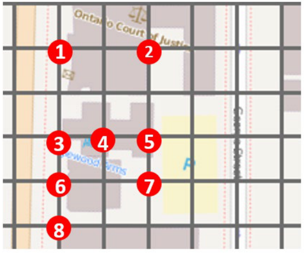
The dots on the Toronto neighborhood map in Figure 29.4 show locations of past cardiac arrests. The city wants to place automated external defibrillators, or AEDs, to cover all eight locations. Each grid square measures 50 m by 50 m. An AED can be placed only at a numbered dot, distances are rectilinear, and the coverage distance is 100 m.
Q1.1 Minimum number of AEDs
Assume an AED costs the same at every location. Find the minimum number of AEDs and give their locations. Show why your solution is optimal.
NoteSolution
The coverage sets are listed in Table 29.21. Each set includes its AED location and every dot within 100 m rectilinear distance.
| AED location | Covered locations |
|---|---|
| 1 | 1, 2, 3 |
| 2 | 1, 2, 5 |
| 3 | 1, 3, 4, 5, 6, 8 |
| 4 | 3, 4, 5, 6, 7 |
| 5 | 2, 3, 4, 5, 7 |
| 6 | 3, 4, 6, 7, 8 |
| 7 | 4, 5, 6, 7 |
| 8 | 3, 6, 8 |
The minimum number of AEDs is 2. The location pairs {2, 6}; {3, 5} are both optimal.
To check the result:
- Verify coverage in Table 29.22. Each pair covers all 8 points.
- Rule out a single AED. One location covers at most 6 of the 8 points.
Either displayed pair therefore attains the minimum possible count.
| AED locations | Number of AEDs |
|---|---|
| 2, 6 | 2 |
| 3, 5 | 2 |
Q1.2 Location-dependent costs
An AED costs $2,000 at locations 1, 3, 6, and 8; $1,500 at locations 4 and 5; and $1,000 at locations 2 and 7. The coverage distance remains 100 m. Apply the weighted greedy rule that selects the smallest cost per newly covered location. Give the selected locations, total cost, and whether the result is optimal.
NoteSolution
Apply the weighted greedy rule in this order:
- Select location 7. Its opening cost per covered point is the smallest, at $250. It covers 4, 5, 6, 7, leaving 1, 2, 3, 8 uncovered.
- Select location 2. It costs $1,000 and covers the new points 1, 2.
- Cover the remaining points 3, 8 with any of the tied locations 3, 6, 8. Each final AED costs $2,000.
Table 29.23 and the following tables give every selection in the tied greedy branches.
| Selection | Newly covered | Cost per new point (dollars) |
|---|---|---|
| 1. Site 7 | 4, 5, 6, 7 | 250.00 |
| 2. Site 2 | 1, 2 | 500.00 |
| 3. Site 3 | 3, 8 | 1,000.00 |
| Selection | Newly covered | Cost per new point (dollars) |
|---|---|---|
| 1. Site 7 | 4, 5, 6, 7 | 250.00 |
| 2. Site 2 | 1, 2 | 500.00 |
| 3. Site 6 | 3, 8 | 1,000.00 |
| Selection | Newly covered | Cost per new point (dollars) |
|---|---|---|
| 1. Site 7 | 4, 5, 6, 7 | 250.00 |
| 2. Site 2 | 1, 2 | 500.00 |
| 3. Site 8 | 3, 8 | 1,000.00 |
The greedy location sets are {7, 2, 3}; {7, 2, 6}; {7, 2, 8}, each costing $4,000. The greedy result is not optimal. Locations 2, 6 cover every point for $3,000.
To prove that this pair is optimal, check the possible AED counts:
- One AED cannot cover every point.
- Every cheaper pair in Table 29.26 leaves at least one point uncovered. The table includes every pair costing less than the proposed solution.
- Three or more AEDs cannot be cheaper. The three smallest opening costs sum to $3,500, already above $3,000.
The proposed pair is feasible, and every cheaper possibility has been ruled out.
| AED locations | Cost ($) | Uncovered locations |
|---|---|---|
| 2, 4 | 2,500 | 8 |
| 2, 5 | 2,500 | 6, 8 |
| 2, 7 | 2,000 | 3, 8 |
| 4, 7 | 2,500 | 1, 2, 8 |
| 5, 7 | 2,500 | 1, 8 |
Exercise 2: An optimal picking tour
CASE STUDY
Apply the Ratliff and Rosenthal algorithm using the configurations and transition tables in M8 Dynamic-programming transitions. The picking area in Figure 29.5 has nine north-south aisles and two east-west aisles. Picking occurs in the seven inner aisles, numbered 1 to 7. The I/O point is at the north end of aisle 4. Distances are rectilinear and measured in cell units. Black cells identify required pick locations. The I/O point is also a required vertex of the closed tour.
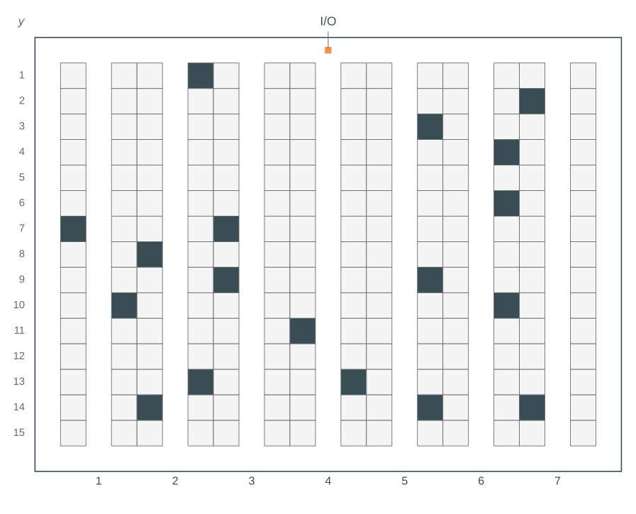
For calculation, Table 29.27 gives the same pick locations numerically. Measure \(y\) downward from the top cross-aisle, so the top and bottom cross-aisles are at \(y=0\) and \(y=16\). Adjacent picking aisles are 3 cell units apart. The depot is at aisle 4, \(y=0\).
| Picking aisle | Required pick coordinates \(y\) |
|---|---|
| 1 | 7, 10 |
| 2 | 1, 8, 13, 14 |
| 3 | 7, 9 |
| 4 | 11, 13 |
| 5 | 3, 9, 14 |
| 6 | 4, 6, 10 |
| 7 | 2, 14 |
Q2.1 Complete the dynamic-programming table
Each entry below gives the minimum partial-tour length, predecessor class number, and added configuration. The five classes are numbered 1 to 5 in the order shown in Table 29.12. The supplied table is divided by aisle for readability. Initialize \(L_1^+\) directly from the within-aisle configurations; dashes at \(L_1^-\) indicate that no predecessor state is used. The records allow a required vertex on the current boundary to remain temporarily unvisited while a later added edge can still reach it. The depot at \(a_4\) must have positive degree before it leaves the boundary. Consequently, the transition from class 3, (0, E, 1C), at \(L_4^+\) using the bottom-only configuration II-iii is infeasible: it would leave the depot unvisited. Configuration II-iv remains available because it also connects the top boundary vertex. Complete entries C and D.
| Class | \(L_1^-\) | \(L_1^+\) |
|---|---|---|
| 1. (U, U, 1C) | - | 16, -, I-i |
| 2. (E, 0, 1C) | - | 20, -, I-ii |
| 3. (0, E, 1C) | - | 18, -, I-iii |
| 4. (E, E, 1C) | - | 32, -, I-v |
| 5. (E, E, 2C) | - | 26, -, I-iv |
| Class | \(L_2^-\) | \(L_2^+\) |
|---|---|---|
| 1. (U, U, 1C) | 22, 1, II-i | C |
| 2. (E, 0, 1C) | 26, 2, II-ii | 54, 2, I-ii |
| 3. (0, E, 1C) | 24, 3, II-iii | 54, 3, I-iii |
| 4. (E, E, 1C) | 44, 4, II-iv | 38, 1, I-i |
| 5. (E, E, 2C) | 30, 3, II-iv | 42, 3, I-iv |
| Class | \(L_3^-\) | \(L_3^+\) |
|---|---|---|
| 1. (U, U, 1C) | 46, 1, II-i | 60, 2, I-i |
| 2. (E, 0, 1C) | 44, 4, II-ii | 62, 2, I-ii |
| 3. (0, E, 1C) | 44, 4, II-iii | 62, 3, I-iii |
| 4. (E, E, 1C) | 50, 4, II-iv | 62, 1, I-i |
| 5. (E, E, 2C) | 54, 5, II-iv | 62, 2, I-iii |
| Class | \(L_4^-\) | \(L_4^+\) |
|---|---|---|
| 1. (U, U, 1C) | 66, 1, II-i | 76, 1, I-iii |
| 2. (E, 0, 1C) | 68, 2, II-ii | 94, 2, I-ii |
| 3. (0, E, 1C) | 68, 3, II-iii | 78, 3, I-iii |
| 4. (E, E, 1C) | 74, 4, II-iv | 82, 1, I-i |
| 5. (E, E, 2C) | 74, 2, II-iv | 78, 2, I-iii |
| Class | \(L_5^-\) | \(L_5^+\) |
|---|---|---|
| 1. (U, U, 1C) | 82, 1, II-i | 102, 1, I-iv |
| 2. (E, 0, 1C) | 88, 4, II-ii | 116, 2, I-ii |
| 3. (0, E, 1C) | 88, 4, II-iii | 114, 3, I-iii |
| 4. (E, E, 1C) | 94, 4, II-iv | 98, 1, I-i |
| 5. (E, E, 2C) | 90, 3, II-iv | 108, 2, I-iv |
| Class | \(L_6^-\) | \(L_6^+\) |
|---|---|---|
| 1. (U, U, 1C) | 108, 1, II-i | 120, 2, I-i |
| 2. (E, 0, 1C) | 104, 4, II-ii | 124, 2, I-ii |
| 3. (0, E, 1C) | 104, 4, II-iii | 128, 3, I-iii |
| 4. (E, E, 1C) | 110, 4, II-iv | 124, 1, I-i |
| 5. (E, E, 2C) | D | 124, 3, I-ii |
| Class | \(L_7^-\) | \(L_7^+\) |
|---|---|---|
| 1. (U, U, 1C) | 126, 1, II-i | 134, 1, I-iv |
| 2. (E, 0, 1C) | 130, 2, II-ii | 158, 2, I-ii |
| 3. (0, E, 1C) | 130, 4, II-iii | 158, 3, I-iii |
| 4. (E, E, 1C) | 136, 4, II-iv | 142, 1, I-i |
| 5. (E, E, 2C) | 136, 2, II-iv | 138, 2, I-iv |
NoteSolution
C is 40, 1, I-iv.
- Start from predecessor class 1 at \(L_2^-\), with length 22.
- Add configuration I-iv, which contributes 18. The total is \(22+18=40\).
- Accept the tied record 40, 3, I-i as well. It reaches the same class with length \(24+16=40\).
D is 120, 5, II-iv.
- Start from predecessor class 5 at \(L_5^+\), with length 108.
- Add configuration II-iv, which contributes 12. The total is \(108+12=120\).
The I/O point at aisle 4, \(y=0\), must be included as a required vertex (Heßler and Irnich 2022, 156). Apply the boundary rule as follows:
- A required vertex may remain temporarily unvisited while it is on the current boundary. It must have positive degree before that boundary is discarded.
- At the depot aisle, a bottom-only connection from class (0, E, 1C) would leave the I/O point unvisited. The recurrence excludes that connection and retains the configuration connecting both boundary vertices.
Q2.2 Draw the optimal tour
Use Figure 29.5 to sketch an optimal closed tour through all required locations.
NoteSolution
At the last aisle, a valid completed tour must satisfy the following conditions:
- It is connected.
- It includes the required depot.
- Every used vertex has even degree (Ratliff and Rosenthal 1983, 513).
Class 4, (E, E, 1C), gives the shortest valid tour, at 142 cell units. The smaller records fail the completion conditions:
- The record with length 134 has odd boundary degrees.
- The record with length 138 has two connected components.
Table 29.35 identifies every admissible terminal state.
| Class | State | Cost | Admissible |
|---|---|---|---|
| 1 | (U, U, 1C) | 134 | No |
| 2 | (E, 0, 1C) | 158 | Yes |
| 3 | (0, E, 1C) | 158 | Yes |
| 4 | (E, E, 1C) | 142 | Yes |
| 5 | (E, E, 2C) | 138 | No |
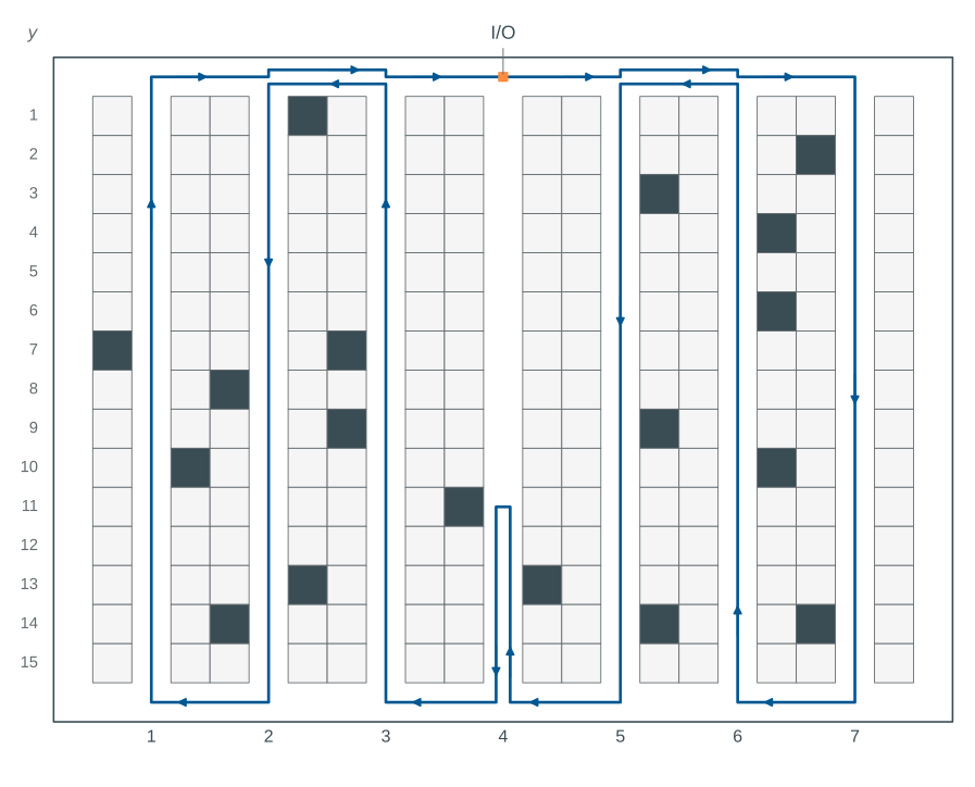
An optimal closed tour of 142 cell units is drawn in Figure 29.6. It starts and finishes at aisle 4, \(y=0\), and visits all 18 required pick locations.
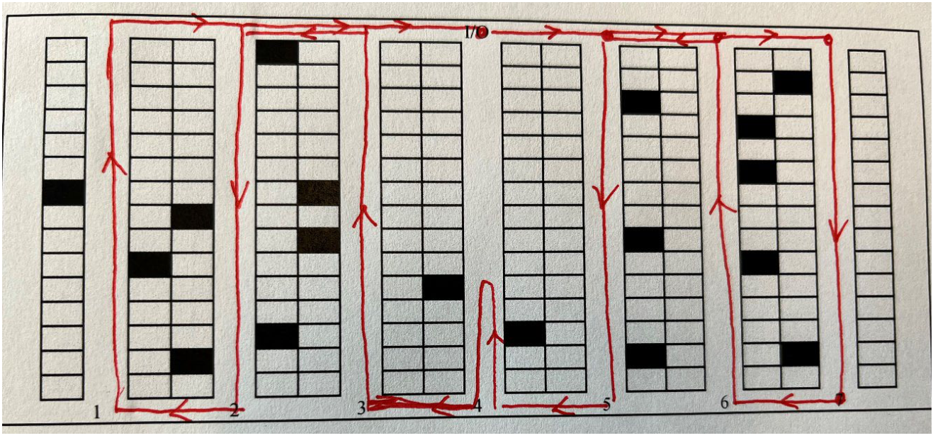
Figure 29.7 shows the same tour on the warehouse blueprint, with separate tracks for repeated travel.
An exact traveling-salesman formulation provides an independent optimality check:
- Use the same required vertices and the two-cross-aisle distance metric (Heßler and Irnich 2022, 156–57).
- Obtain a lower bound of 142 cell units.
- Compare that bound with the feasible tour length. The lengths agree, proving optimality.
Table 29.36 compares the completed tour lengths and lower bounds.
| Method | Tour length | Lower bound | Optimality gap | Feasible closed tour |
|---|---|---|---|---|
| Dynamic programming | 142 | 142 | 0 | Yes |
| Exact traveling-salesman formulation | 142 | 142 | 0 | Yes |
Q2 Cobot-routing formulation
The e-commerce company UTcom has an AGV-assisted warehouse in which cobots act as pickers. Each cobot leaves the single depot, visits pick locations, and returns to the depot. Incoming orders contain one order line. The required pick locations are given, and each must be visited exactly once by the fleet. Assume the cobots can pick and carry the stated items. All cobots have the same capacity, measured in picking items. Assign locations to cobots and sequence their visits to minimize total travel cost.
Use the sets, parameters, and variables in Table 29.37. Complete the objective and the four constraint groups described below. Omit subtour-elimination constraints for this formulation.
| Symbol | Meaning |
|---|---|
| \(N=\{0,1,\ldots,n\}\) | Nodes, with depot 0 and pick locations 1 to \(n\) |
| \(A\subseteq\{(i,j)\in N\times N:i\ne j\}\) | Available directed travel arcs; self-arcs are excluded |
| \(d_i\) | Number of picking items at pick location \(i\in N\setminus\{0\}\) |
| \(c_{ij}\) | Cost of traversing arc \((i,j)\in A\) |
| \(K\) | Number of cobots |
| \(C\) | Maximum number of picking items carried by a cobot |
| \(y_{ik}\) | 1 if cobot \(k\) visits node \(i\), and 0 otherwise |
| \(x_{ijk}\) | 1 if cobot \(k\) travels directly from \(i\) to \(j\), and 0 otherwise |
The required constraint groups ensure that each pick location is visited exactly once, every cobot leaves the depot, travel is conserved at visited nodes, and each route respects capacity.
NoteSolution
For cobots \(k\in\{1,\ldots,K\}\), minimize
\[ \sum_{k=1}^{K}\sum_{(i,j)\in A}c_{ij}x_{ijk}. \]
- Visit each pick location exactly once.
\[ \sum_{k=1}^{K}y_{ik}=1 \qquad\forall i\in N\setminus\{0\}. \]
- Require every cobot to leave the depot.
\[ \sum_{j:(0,j)\in A}x_{0jk}=1 \qquad\forall k\in\{1,\ldots,K\}. \]
- Conserve travel and link it to node visits.
\[ \sum_{j:(i,j)\in A}x_{ijk} =\sum_{j:(j,i)\in A}x_{jik} =y_{ik} \qquad\forall i\in N,\ k\in\{1,\ldots,K\}. \]
At node 0, these equalities also require one return to the depot for each cobot.
- Limit the picking load.
\[ \sum_{i\in N\setminus\{0\}}d_i y_{ik}\leq C \qquad\forall k\in\{1,\ldots,K\}. \]
Use binary domains for every defined \(x_{ijk}\) and \(y_{ik}\).
The formulation shown is a partial vehicle-routing model. Without the omitted subtour-elimination constraints, the equations can admit disconnected cycles and do not alone establish valid depot-connected routes.
Numerical illustration. Consider one cobot and the small instance in Table 29.38. Distances are rectilinear and capacity is 3 items.
These values illustrate the formulation; they are not additional data for the question.
| Node | x | y | Demand (items) |
|---|---|---|---|
| 0 | 0 | 0 | 0 |
| 1 | 1 | 0 | 1 |
| 2 | 10 | 0 | 1 |
| 3 | 11 | 0 | 1 |
Compare the results:
- The partial model has minimum cost 4 and admits the cycles in Table 29.39.
- A separate enumeration of every cycle cover confirms that minimum.
- The shortest depot-connected tour costs 22.
The difference shows why the omitted connectivity constraints matter.
| Cobot | Cycle | Contains depot |
|---|---|---|
| 1 | 0 → 1 → 0 | Yes |
| 1 | 2 → 3 → 2 | No |
Exercise 3: Departmental layout
CASE STUDY
Three departments, D1, D2, and D3, are squares with side length \(a>0\). Place them without overlap in a building of length \(5a\) and width \(a\). Touching boundaries are allowed. The exercise concerns qualitative preferences for proximity or separation.
Q3.1 Interpret preference weights
Propose an integer scale for the preferences “strongly prefer proximity”, “prefer proximity”, “indifferent”, “prefer separation”, and “strongly prefer separation”. The objective is minimized and multiplies each weight by the distance between department centroids. Explain the signs in your scale.
NoteSolution
Following the preference order in the question, one possible scale is 2, 1, 0, -1, -2. Interpret the signs in the minimized objective as follows:
- A positive weight penalizes separation.
- Zero gives no distance contribution.
- A negative weight rewards separation.
Other scales with the same stated interpretation are possible. The weights express qualitative preferences in a bounded layout exercise.
The objective measures a preference score. Physical flows and monetary handling costs would require different input data.
Table 29.40 shows how each weight changes the minimized score when centroid distance increases.
| Preference | Weight | Score at distance 1 | Score at distance 2 | Change in score |
|---|---|---|---|---|
| Strongly prefer proximity | 2 | 2 | 4 | 2 |
| Prefer proximity | 1 | 1 | 2 | 1 |
| Indifferent | 0 | 0 | 0 | 0 |
| Prefer separation | -1 | -1 | -2 | -1 |
| Strongly prefer separation | -2 | -2 | -4 | -2 |
For the remaining parts, use the fixed weights in Table 29.41, regardless of the scale you proposed.
| Department pair | Preference | Weight \(w_{ij}\) |
|---|---|---|
| D1, D2 | Indifferent | 0 |
| D1, D3 | Strongly prefer separation | -2 |
| D2, D3 | Strongly prefer separation | -2 |
Use the following fixed-dimension department-layout model. For department \(i\in\{1,2,3\}\), let \(x_i^L,x_i^R,y_i^B,y_i^T\) be its left, right, bottom, and top coordinates. Its centroid is \((\alpha_i,\beta_i)\). The geometric constraints are
\[ \begin{aligned} &x_i^R-x_i^L=a,\qquad y_i^T-y_i^B=a &&\forall i,\\ &0\leq x_i^L,\qquad x_i^R\leq5a &&\forall i,\\ &0\leq y_i^B,\qquad y_i^T\leq a &&\forall i,\\ &\alpha_i=(x_i^L+x_i^R)/2,\qquad \beta_i=(y_i^B+y_i^T)/2 &&\forall i. \end{aligned} \]
For each ordered pair \(i\ne j\), let binary \(z^x_{ij}=1\) enforce that \(i\) lies left of \(j\), and \(z^y_{ij}=1\) enforce that \(i\) lies below \(j\). With \(M=5a\), nonoverlap is imposed by
\[ \begin{aligned} &x_i^R\leq x_j^L+M(1-z^x_{ij}) &&\forall i\ne j,\\ &y_i^T\leq y_j^B+M(1-z^y_{ij}) &&\forall i\ne j,\\ &z^x_{ij}+z^x_{ji}+z^y_{ij}+z^y_{ji}\geq1 &&\forall i<j,\\ &z^x_{ij},z^y_{ij}\in\{0,1\} &&\forall i\ne j. \end{aligned} \]
Minimize the score
\[ S=\sum_{i<j}w_{ij} \left(|\alpha_i-\alpha_j|+|\beta_i-\beta_j|\right). \]
Retain the exact absolute values; no linearization is required. The displayed objective is not linear. Replacing an absolute value only by a lower-bounding distance variable would be invalid when its coefficient is negative.
Q3.2 Find an optimal layout
Draw an optimal layout, give its centroid distances, and calculate its score. Show why the score is optimal.
NoteSolution
Every square fills the building’s width, so all centroid coordinates satisfy \(\beta_i=a/2\). The arrangement in Figure 29.8 places D1 and D2 at one end and D3 at the other. Table 29.42 gives the coordinates as multiples of \(a\).
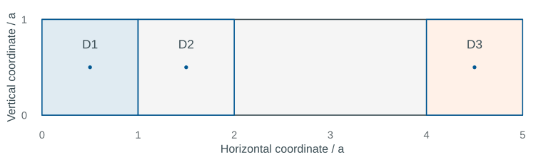
| Department | Left / a | Right / a | Centroid x / a |
|---|---|---|---|
| D1 | 0 | 1 | 0.5 |
| D2 | 1 | 2 | 1.5 |
| D3 | 4 | 5 | 4.5 |
The pairwise distances and score contributions are given in Table 29.43. Each unordered department pair is counted once.
| Pair | Distance / a | Weight | Score / a |
|---|---|---|---|
| D1, D2 | 1 | 0 | 0 |
| D1, D3 | 4 | -2 | -8 |
| D2, D3 | 3 | -2 | -6 |
The normalized score \(S/a\) is -14. To prove optimality, consider D3’s position in the department order:
- D3 is at an end. The two farthest feasible other centroids are 4\(a\) and 3\(a\) away. Their distance sum is at most 7\(a\).
- D3 is between the other departments. The distance sum is at most the building’s 4\(a\) centroid span.
The displayed arrangement attains the larger bound. Since both nonzero weights are negative and equal, attaining that bound minimizes the score.
\[S=- 14 a.\]
Swapping D1 and D2, or reflecting the arrangement, gives other optimal layouts before the locations are fixed. Table 29.44 checks every possible department order.
| Department order | Minimum score / a |
|---|---|
| D1–D2–D3 | -14 |
| D1–D3–D2 | -8 |
| D2–D1–D3 | -14 |
| D2–D3–D1 | -8 |
| D3–D1–D2 | -14 |
| D3–D2–D1 | -14 |
The exact absolute-value objective is necessary for these signed preference weights. The auxiliary-distance linearization in Tompkins et al. (2010, 327–30) assumes nonnegative coefficients.
With negative coefficients, lower bounds alone do not force an auxiliary distance to equal the actual centroid distance.
Q3.3 Fix department locations
How can the model fix D1 at the left end and D3 at the right end of the building?
NoteSolution
Fix D1’s left boundary and D3’s right boundary with the following equalities.
\[x_1^L=0,\qquad x_3^R=5a.\]
The fixed square side lengths determine the other horizontal boundaries and centroids, as shown in Table 29.45. All vertical centroids remain at \(a/2\).
| Department | Left / a | Right / a | Centroid x / a |
|---|---|---|---|
| D1 | 0 | 1 | 0.5 |
| D2 | 1 | 2 | 1.5 |
| D3 | 4 | 5 | 4.5 |
The displayed optimal layout satisfies these constraints. The fixed-location model therefore retains the normalized optimum \(S/a=\) -14.
For the department nonoverlap and centroid model, see Tompkins et al. (2010, 327–30).
Q3 Floor-space requirements
An SKU has the inventory-management characteristics in Table 29.46.
Derive its estimated floor-space requirement in square feet using the supplied parameters.
| Parameter | Characteristic | Example |
|---|---|---|
| \(D\) | Forecast annual demand (units/year) | 275,629 |
| \(r\) | Forecast unit turn rate (per year) | 6.2 |
| \(n\) | Units per pallet | 43 |
| \(a\) | Peak-to-average inventory ratio | 108% |
| \(b\) | Percentage of peak used for planning | 92% |
| \(c\) | Maximum pallet-location utilization | 80% |
| \(p\) | Floor area per pallet position (ft²) | 10.14 |
NoteSolution
The formula gives a continuous planning estimate of floor area. A physical design must specify how pallet positions and complete rack modules are rounded.
Use the supplied density of 10.14 ft² per pallet position throughout this question. That value is an independent planning input.
Calculate the continuous estimate in this order:
- Divide annual demand by the turnover rate to estimate average inventory, \(\bar I\).
- Divide average inventory by units per pallet to obtain average pallets on hand.
- Multiply by the peak-to-average ratio and planning percentage, then divide by location utilization. The result is the required pallet-position estimate.
- Multiply by the floor area per pallet position.
Combining the steps gives
\[ A=\frac{Dabp}{rnc}. \]
Table 29.47 shows every calculation, including the turnover consistency check. Retain full precision in intermediate values and apply no integer rounding to the continuous estimate.
| Quantity | Formula | Unit | Value |
|---|---|---|---|
| Unit turn rate | \(D/\bar I\) | 1/year | 6.20 |
| Average inventory | \(D/r\) | units | 44,456.29 |
| Average pallets on hand | \(D/(rn)\) | pallets | 1,033.87 |
| Peak pallet inventory | \(Da/(rn)\) | pallets | 1,116.58 |
| Planned pallet capacity | \(Dab/(rn)\) | pallets | 1,027.25 |
| Required pallet positions | \(Dab/(rnc)\) | positions | 1,284.06 |
| Floor area | \(Dabp/(rnc)\) | ft² | 13,020.40 |
Using the supplied values gives
\[\frac{Dabp}{rnc}=\frac{275629\cdot1.08\cdot0.92\cdot10.14}{6.20\cdot43\cdot0.80}\approx 13{,}020.40\ \mathrm{ft}^2.\]
If whole pallet positions are required:
- Round the continuous estimate of 1,284.06 upward to 1,285 positions.
- Calculate area using that whole-position count. The corresponding estimate is 13,029.90 ft².
Complete rack modules may require further rounding.
Q4 Single-deep storage geometry
A warehouse designer must determine the space requirements of a unit-load storage department for one SKU. Management has already chosen the handling and storage systems. The settings are listed in Table 29.48, and the single-deep storage-unit geometry is shown in Figure 29.9.
| Parameter | Description | Example |
|---|---|---|
| \(p_W\) | Pallet width (in) | 40 |
| \(p_L\) | Pallet length (in) | 48 |
| \(p_H\) | Loaded pallet height (in) | 48 |
| \(a\) | Clear height (ft) | 21 |
| \(b\) | Aisle width (in) | 144 |
| \(c\) | Number of levels | 4 |
| \(d\) | Pallet space (in) | 4 |
| \(r\) | Rack-upright width (in) | 3 |
| \(o\) | Lift-off allowance (in) | 4 |
| \(e\) | Beam height (in) | 3 |
| \(f\) | Clear flue space (in) | 6 |
| \(n\) | Pallet footprints per storage unit | 4 |
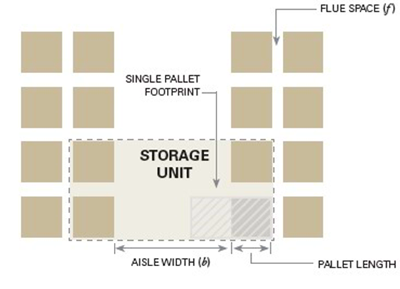
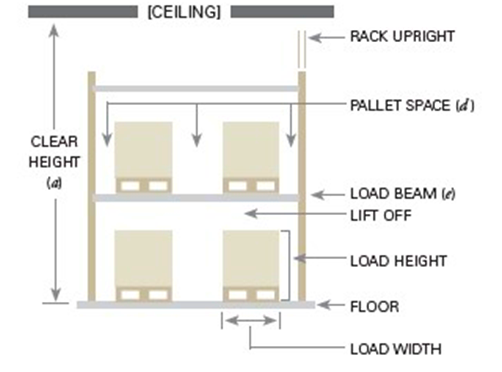
Give formulas for storage-unit depth \(u_d\), storage-unit width \(u_w\), storage-unit floor area \(u_{sf}\), area per pallet footprint \(u_{fp}\), area per pallet position \(p\), and minimum height \(h\). Use the stated convention of a pallet height, lift-off allowance, and beam height at each of the \(c\) levels.
| Parameter | Description | Calculation formula |
|---|---|---|
| \(u_{\mathrm{d}}\) | Storage unit depth/length (in) | |
| \(u_{\mathrm{w}}\) | Storage unit width (in) | |
| \(u_{\mathrm{sf}}\) | Sq. ft. of storage unit | |
| \(u_{\mathrm{fp}}\) | Sq. ft. per pallet footprint | |
| \(p\) | Sq. ft. per pallet position | |
| \(h\) | Min. height (in) |
NoteSolution
The calculations are given in Table 29.50.
| Quantity | Formula | Unit | Value |
|---|---|---|---|
| Unit depth | \(b+2p_L+f\) | in | 246.00 |
| Unit width | \(2p_W+3d+r\) | in | 95.00 |
| Unit floor area | \(u_du_w/144\) | ft² | 162.29 |
| Area per pallet footprint | \(u_{sf}/n\) | ft² | 40.57 |
| Area per pallet position | \(u_{fp}/c\) | ft² | 10.14 |
| Minimum height | \(c(p_H+o+e)\) | in | 220.00 |
- The divisor 144 converts square inches to square feet because one foot is 12 inches.
- The unit has 4 pallet footprints and 4 levels, giving 16 pallet positions.
- Before rounding to two decimals, the density is approximately 10.143229 ft² per position.
The inventory floor-space question supplies its own density; rounding this geometry result does not replace that independent input.
Under the stated per-level beam and clearance convention, the required height is
\[h=c(p_H+o+e)=4\left(48+4+3\right)=220\ \mathrm{in}.\]
Check the height requirement:
- Available clear height is 252 inches.
- Required height is 220 inches, leaving 32 inches of clearance.
The stated geometry therefore fits the height assumption. The beam and clearance convention is part of the supplied example and must be checked against the intended rack design in practice.
Q5 Automated retail material flow
The following activities describe a particular automated retail-warehouse flow, but appear in the wrong order.
- Selected suppliers unload their own trucks and feed preannounced single-SKU pallets to a check-in conveyor.
- Pallets or roll cages wait in an order-consolidation buffer, usually an AS/R system.
- Pallets are offloaded and automatically destacked by robots.
- When a store order arrives, cases are retrieved and sequenced.
- Mixed-case palletizers build pallets or roll cages in a store-specific sequence that allows rapid shelving in the store.
- Loose cases are stored in a miniload AS/R or an AVS/R system.
- Pallets are stored in an AS/R system.
- Pallets or roll cages are retrieved and loaded in the sequence determined by the stops on the truck route.
Give the correct sequence of activity numbers.
NoteSolution
The sequence is 1, 7, 3, 6, 4, 5, 2, 8. Follow the material through the warehouse:
- Receive inbound single-SKU pallets on the conveyor and place them in pallet AS/R storage.
- Retrieve and destack pallets, then place the loose cases in case storage.
- For a store order, retrieve and sequence cases, then assemble mixed pallets or roll cages.
- Hold completed loads in the consolidation buffer, then retrieve and load them in route-stop sequence.
Azadeh et al. (2019, 918) describes this retail-automation example.
Table 29.51 connects each activity number to its chronological step.
| Step | Activity number | Activity |
|---|---|---|
| 1 | 1 | Check in inbound pallets |
| 2 | 7 | Store inbound pallets |
| 3 | 3 | Retrieve and destack pallets |
| 4 | 6 | Store loose cases |
| 5 | 4 | Retrieve and sequence cases |
| 6 | 5 | Build store-specific mixed loads |
| 7 | 2 | Consolidation buffer |
| 8 | 8 | Retrieve and load the truck |
References
Azadeh, Kaveh, René de Koster, and Debjit Roy. 2019. “Robotized and Automated Warehouse Systems: Review and Recent Developments.” Transportation Science 53 (4): 917–45. https://doi.org/10.1287/trsc.2018.0873.
Bahrami, Behnam, Hemen Piri, and El-Houssaine Aghezzaf. 2019. “Class-Based Storage Location Assignment: An Overview of the Literature:” Proceedings of the 16th International Conference on Informatics in Control, Automation and Robotics (Prague, Czech Republic), 390–97. https://doi.org/10.5220/0007952403900397.
Frazelle, Edward. 2016. World-Class Warehousing and Material Handling. Second Edition. McGraw-Hill Education.
Heragu, Sunderesh S. 2022. Facilities Design. Fifth edition. CRC Press.
Heßler, Katrin, and Stefan Irnich. 2022. “A Note on the Linearity of Ratliff and Rosenthal’s Algorithm for Optimal Picker Routing.” Operations Research Letters 50 (2): 155–59. https://doi.org/10.1016/j.orl.2022.01.014.
Koster, René de, Tho Le-Duc, and Kees Jan Roodbergen. 2007. “Design and Control of Warehouse Order Picking: A Literature Review.” European Journal of Operational Research 182 (2): 481–501. https://doi.org/10.1016/j.ejor.2006.07.009.
Liu, Xiulong, Jiannong Cao, Yanni Yang, and Shan Jiang. 2018. “CPS-Based Smart Warehouse for Industry 4.0: A Survey of the Underlying Technologies.” Computers 7 (1, 1): 13. https://doi.org/10.3390/computers7010013.
Ratliff, H. Donald, and Arnon S. Rosenthal. 1983. “Order-Picking in a Rectangular Warehouse: A Solvable Case of the Traveling Salesman Problem.” Operations Research 31 (3): 507–21. https://doi.org/10.1287/opre.31.3.507.
Tompkins, James A., John A. White, Yavuz A. Bozer, and J. M. A. Tanchoco. 2010. Facilities Planning. 4th ed. John Wiley & Sons. https://www.wiley-vch.de/en/areas-interest/engineering/facilities-planning-978-0-470-44404-7.
Zhen, Lu, and Haolin Li. 2022. “A Literature Review of Smart Warehouse Operations Management.” Frontiers of Engineering Management 9 (1): 31–55. https://doi.org/10.1007/s42524-021-0178-9.